Performance Tuning of the Hazelcast SQL Engine

In Hazelcast Platform 5.1 contains two querying APIs:

• Predicate API
• SQL engine

Predicate API is an older Java-based API. Even though it contains sqlPredicate, which allows using SQL-like syntax for the WHERE clause, the syntax is non-standard, for example NULL handling doesn’t support the (in)famous ternary logic. It fetches the results in one batch, which limits the  supported result size.

On the other hand, SQL Engine is a more modern engine, it uses standard SQL, a cost-based optimizer, and is available in all programming languages. It also supports JOIN, ORDER BY, GROUP BY or UNION operators, which don’t have an equivalent in the Predicate API. It streams the results to the client, so the result size isn’t limited (though this is also a restriction, because it’s not possible to restart the query if it fails mid-way).

In the next major release, we plan to deprecate the Predicate API. For this, we need feature parity and match Predicate API’s performance. The performance is the focus of this blog post: we’ll describe our journey in benchmarking and fixing some performance issues we had.

Benchmark details

Here is a list of benchmarks that we did for that comparison:

	SQL	Predicate API
1	SELECT __key, this FROM iMap	map.entrySet()
2	SELECT count(*) FROM iMap SELECT count(__key) FROM iMap	map.aggregate(Aggregators.count())
3	SELECT sum(\"value\") FROM iMap	map.aggregate(Aggregators.longSum("value"))
4	SELECT sum(JSON_VALUE(this, '$.value' RETURNING INTEGER)) FROM iMap	map.aggregate(Aggregators.longSum("value"))
5	SELECT __key, this FROM iMap WHERE \"value\" = ?	map.entrySet(Predicates.equal("value", valueMatch))

The fifth benchmark was run with and without index on value field. For benchmark number three, we used three different serialization methods:

• IdentifiedDataSerializable
• Portable
• HazelcastJsonValue with json-flat SQL mapping

For the rest of the benchmarks, we used IdentifiedDataSerializable. If you are not familiar with our serialization options check this page.

We didn’t benchmark joins and streaming queries since they cannot be executed with Predicate API. These functionalities are available in the SQL engine only.

Testing environment

All the benchmarks were run in throughput and latency modes since we cared about both. In this post, I will cover only the latency part of those benchmarks.

The first results showed that the SQL was slower in most of them. The next step was to rerun those benchmarks with the attached profiler. I used Async-profiler, and since I was tracing latency issues, I chose wall-clock mode. You can read about different modes in my previous post.

All of those benchmarks were run in our testing lab, so we knew that the results were valid (no noisy-neighbor issue). The setup for the models was:

• Hazelcast cluster size: 4
• Machines with Intel Xeon CPU E5-2687W
• Heap size: 10 GB
• JDK17

How does Hazelcast SQL work?

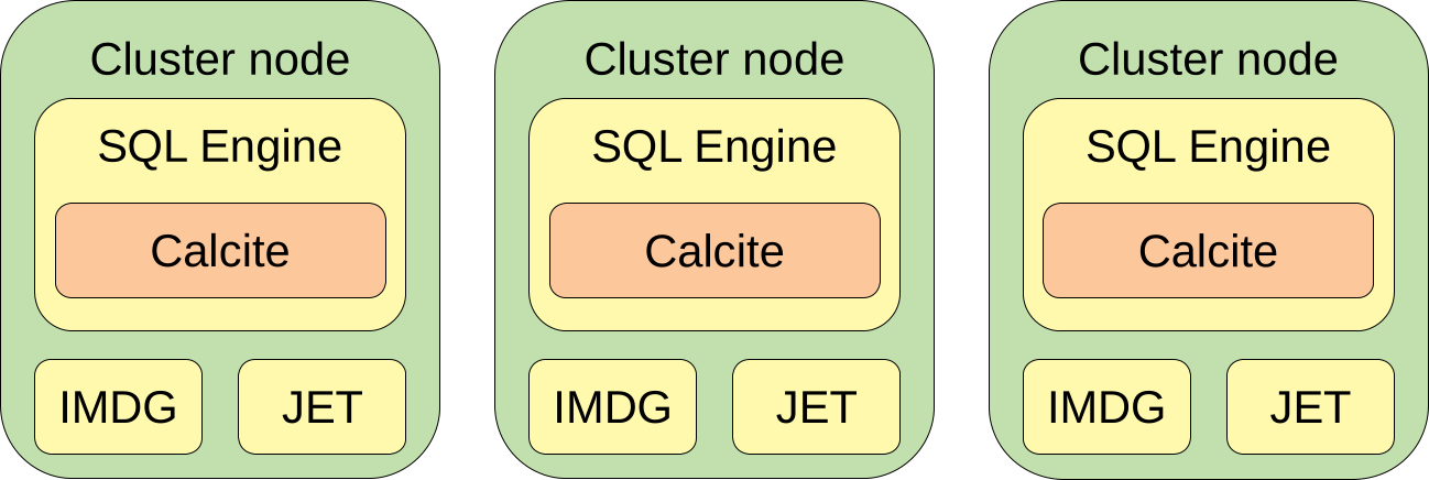
Each of the cluster members contains two significant modules: IMDG and JET. IMDG is a module where we store our data. JET is a distributed batch and stream processing engine. Additionally, for parsing the SQL queries we use Apache Calcite.

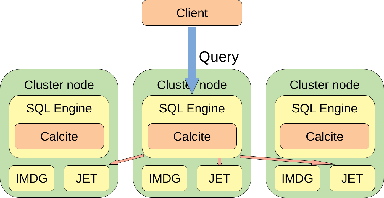
When a client sends a query to a cluster, that query is just a string with parameters. The query is sent to a random member of the cluster. That member is called a coordinator of that query. The coordinator needs to:

• Create a query plan
• Convert the query plan to the JET job
• Distribute the JET job to all the members

After that is done, all the members execute the query, and the coordinator to the client streams the results.

Flame graphs

If you do sampling profiling you need to visualize the results. The results are nothing more than a set of stactraces. My favorite way of visualization is a flame graph. The easiest way to understand what flame graphs are is to know how they are created.

First part is to draw a rectangle for each frame of each stactrace. The stactraces are drawn bottom-up and sorted alphabetically. For example, such a graph:

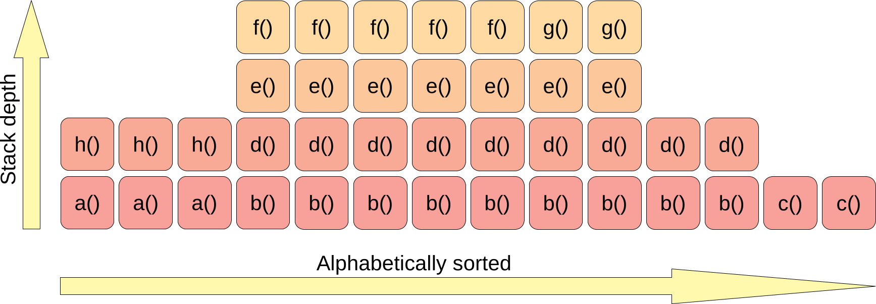
corresponds to set of stactraces:

• 3 samples – a() -> h()
• 5 samples – b() -> d() -> e() -> f()
• 2 samples – b() -> d() -> e() -> g()
• 2 samples – b() -> d()
• 2 samples – c()

The next step is joining the rectangles with the same method name to one bar:

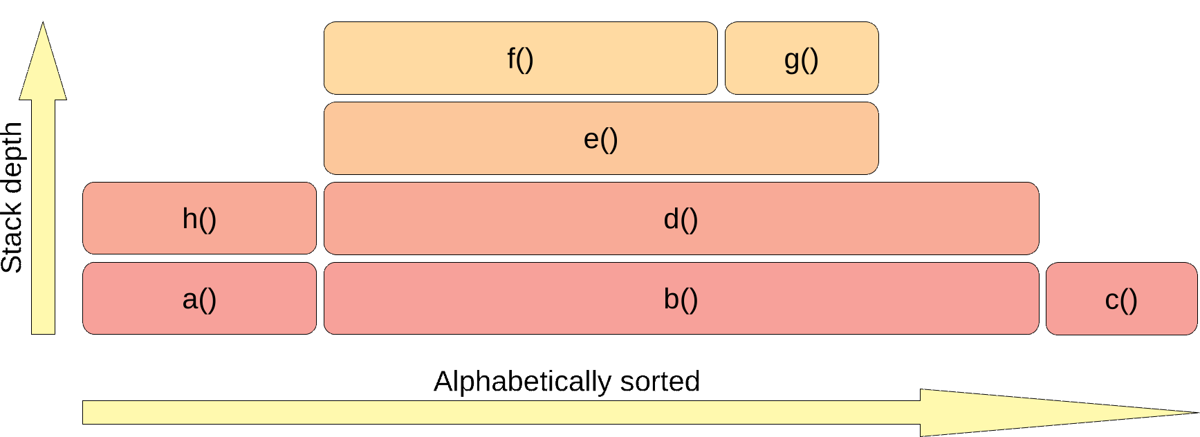
The flame graph usually shows you how your application utilizes some resource. The resource is used by the top methods of that graph (visualized with a green bar):

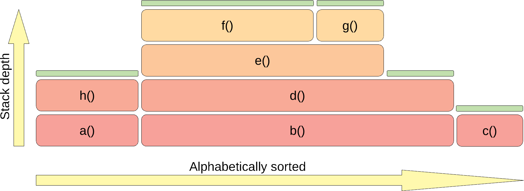
So in this example, method b() is not utilizing the resource at all; it just invokes methods that do it. Flame graphs are commonly used to present the CPU utilization, but the CPU is just one of the resources that we can visualize this way. If you use wall-clock mode then your resource is time. If you use allocation mode then your resource is a heap.

Client part

Benchmark details:

• Query: SELECT __key, this FROM IMap
• Values in IMap have fields: String and int[20], serialized with IdentifiedDataSerializable
• IMap size – 100_000 entries
• Latency test – 24 queries per second

Let’s start with profiling the client side. Here is a wall-clock flame graph of the method that fetches the data on the client’s side:

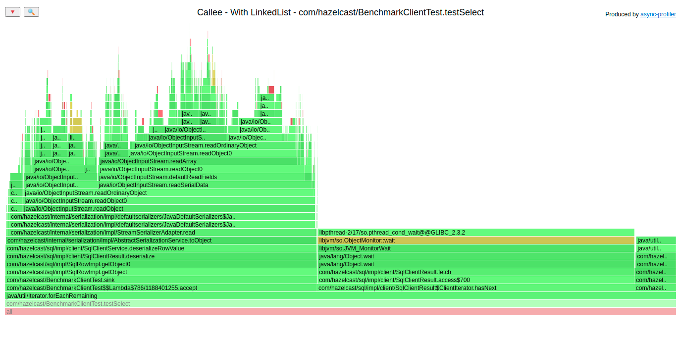
Let’s look at the bottom of the flame graph, method testSelect() iterates over the results and for each row, it executes three things:

• Method accept() – that executes the deserialization of the row – each SQL row travels to the client through the network as a byte array, so we need to deserialize it to the object format
• Method ClientIterator.hasNext() – that one returns the next row if it is already fetched or waits to receive the next portion of the result set. In the flame graph, we see the waiting part. At this point the execution is done in the cluster – nothing to improve on the client’s side.
• Some third method, let’s zoom in on that part of the flame graph

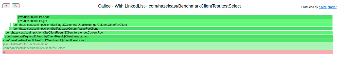
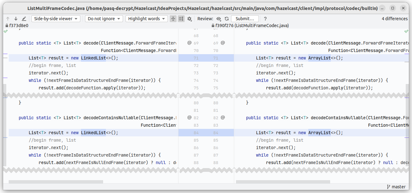
Here we can see that the method getColumnValueForClient() (3rd from the top) executes LinkedList.get() which consumes a lot of time. Let’s go to the source code:

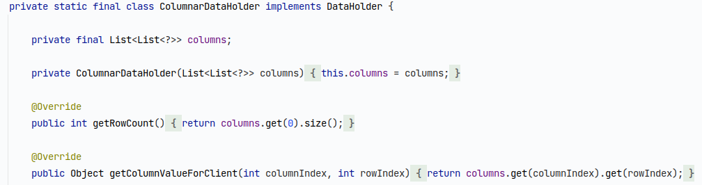
columns is a field of type List<List<?>>, and the problematic method executes columns.get(columnIndex).get(rowIndex). Executing LinkedList.get(index) is known to have a bad performance, since it has O(size) complexity. The instance is not created here; it is passed in the constructor, so we need to debug the application to find the origin of that LinkedList. Two breakpoints later, I found a place where it was created. One solution is to switch that List to ArrayList like this:

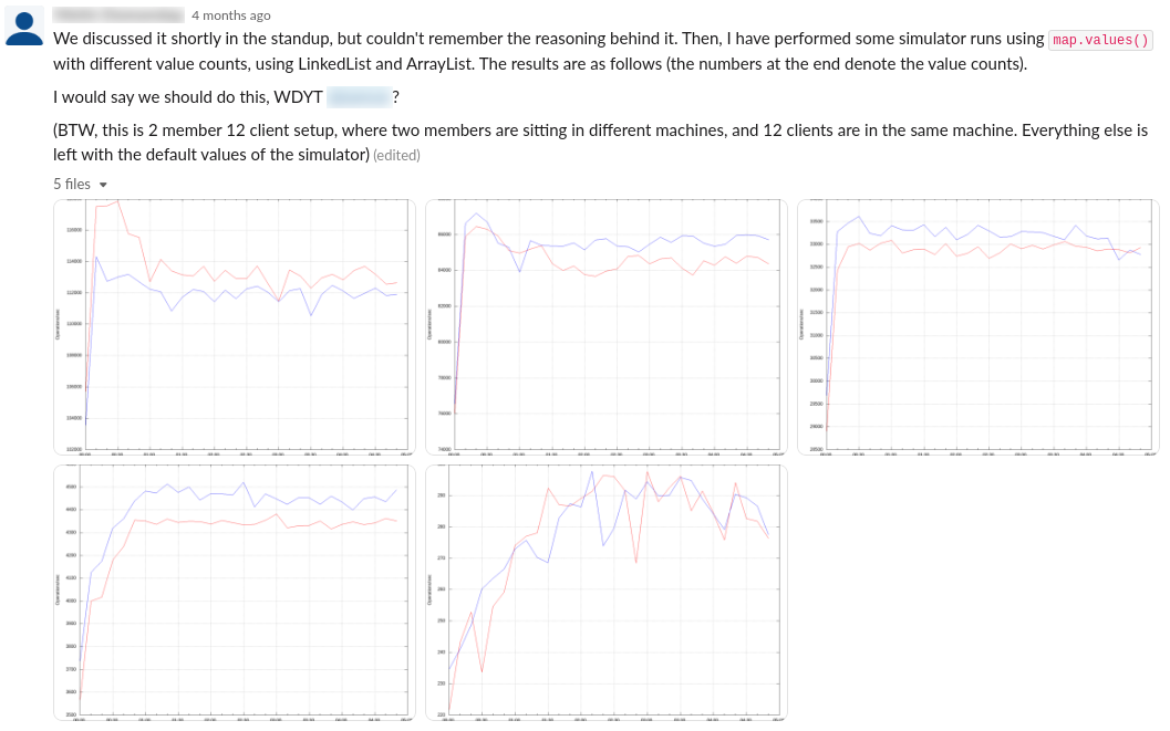
But it is not always that easy. The code where that list was created was done many years ago and is used not only by the SQL engine. We need to be careful here. I asked colleagues from the other team if we could do it, and they did their benchmarks and agreed to that change:

How did that affect our performance? Well, it depends on the number of columns and whether we do deserialization on the client’s side (it is done lazily). Here is the latency distribution for two columns and no deserialization:

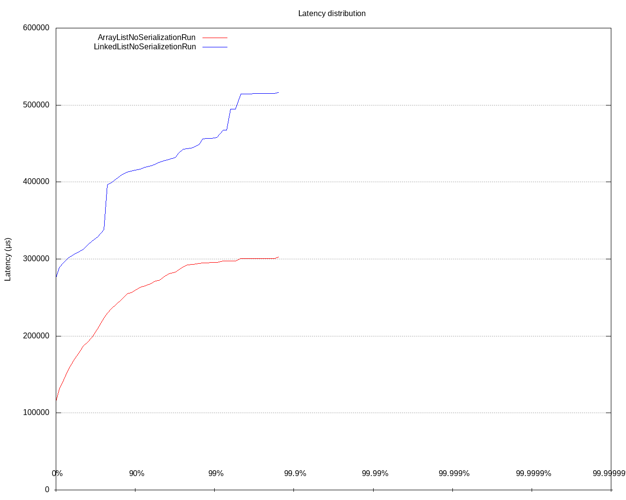
Was it a mistake to choose LinkedList in that code? No. It was a coherent decision made by the state of Hazelcast at the moment of creation of that code.

The thing to remember is that performance is a living organism. It evolves with new features. What was efficient yesterday could be a bottleneck tomorrow.

PR: https://github.com/hazelcast/hazelcast/pull/20398

Cluster side – sum()

Benchmark details:

• Query: SELECT sum(”value”) FROM IMap
• Values in IMap have fields: one Long, and one in[20], serialized with IdentifiedDataSerializable
• IMap size – 1_000_000 entries
• Latency test – 6 queries per second

In this benchmark, we need to deserialize all the instances in IMap, get a single field from that deserialized object, and aggregate it. The majority of work is deserialization. It was strange to me that the Predicate API performed differently than SQL.

Here is a flame graph for Predicate API:

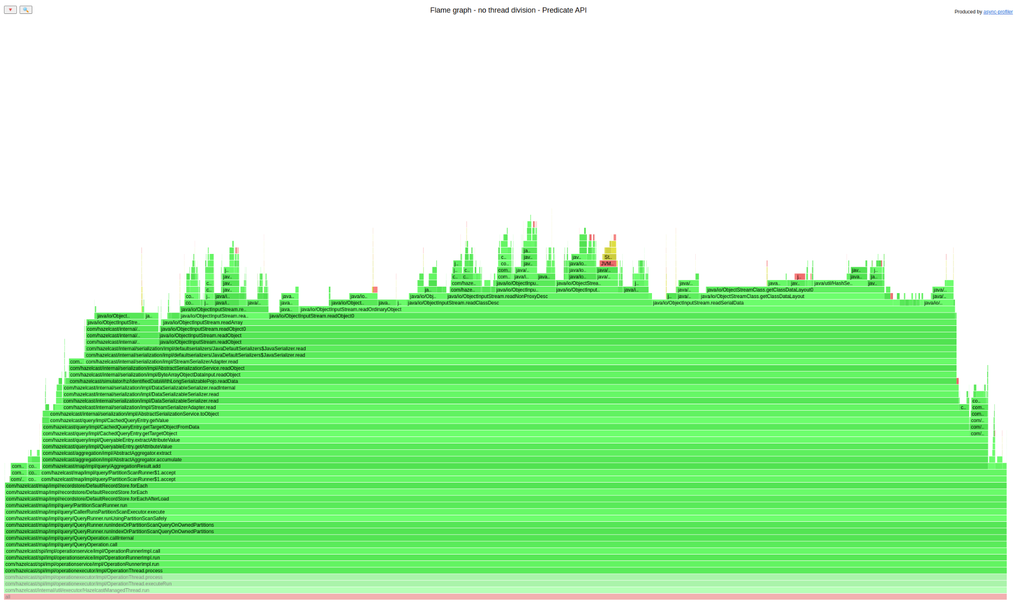
And here is one for SQL:

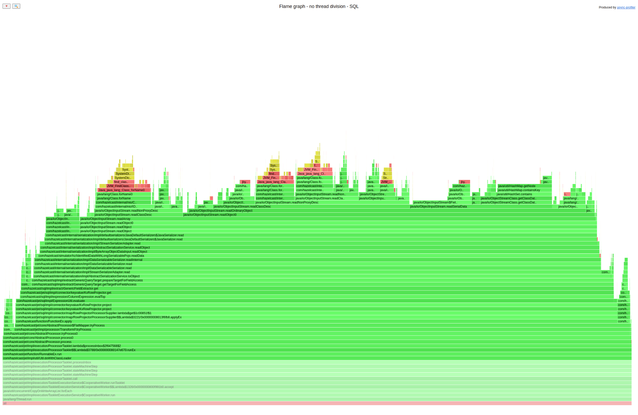
Now let’s do something a bit silly. Open both graphs in separate browser tabs (right mouse click on the graph -> open graphics in a new tab) and then just switch between those two tabs very quickly and try to find a difference. Did you spot it? It is at the top. The SQL graph has a lot of yellow/red code there; the Predicate API does not. Let’s see what it is about:

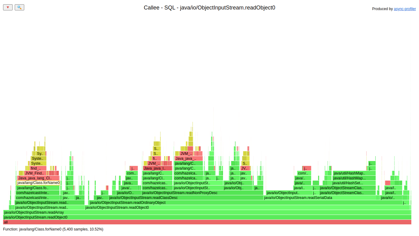
The frames that we can see in SQL only are Class.forName(). We already had a class definition cache in Hazelcast, and it was strange that it wasn’t used for SQL. We can highlight all invocations of that method to see how much time it consumes:

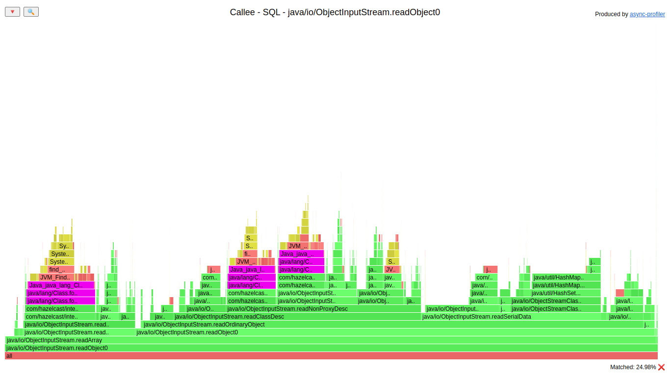
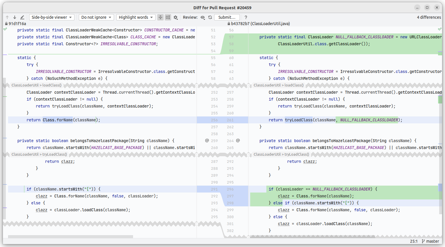
So loading of classes consumed ~25% of the deserialization of Java objects. Let’s look at the code of our class loading:

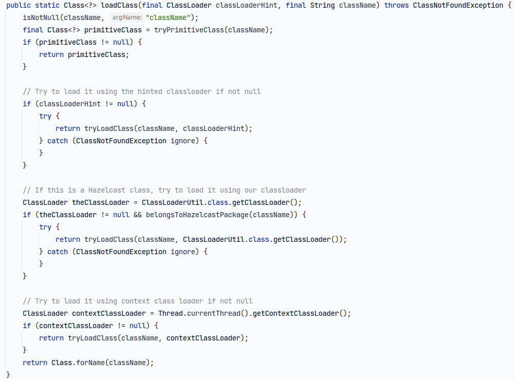
We have four layers of caches here; each tryLoadClass() checks if the definition is in the cache; if not it loads it. If none of the classloaders loaded the class we called Class.forName().

The difference between Predicate API and SQL was that the contextClassLoader was null in SQL since you cannot use user classes with SQL queries. We decided to add another level of cache:

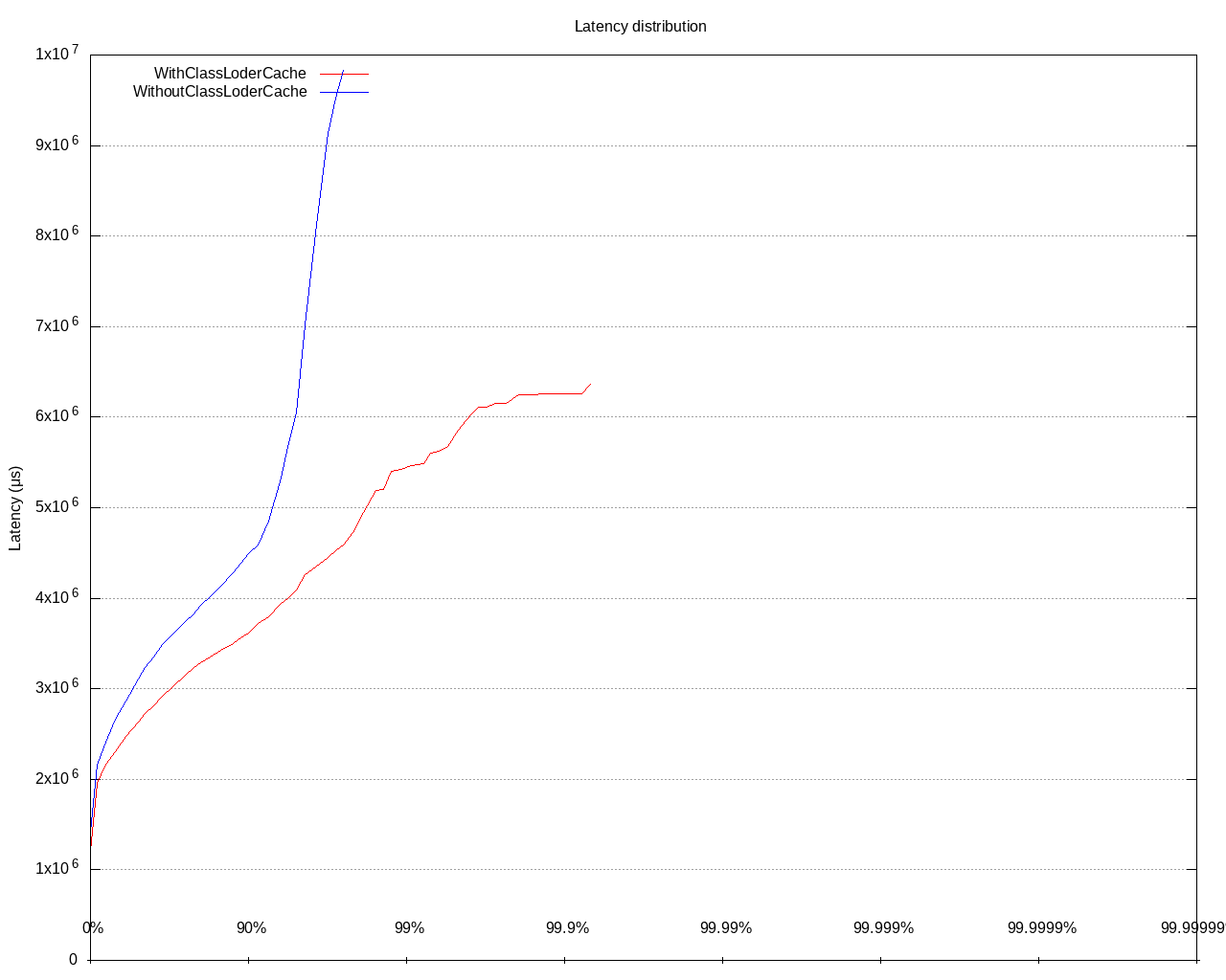
How did that improve the performance?

The thing to remember is that “If it looks stupid but works, it isn’t stupid” – that also applies to the performance analysis. Comparing two flame graphs by quickly switching the browser tabs looks silly, but hey, it works like a charm. If you want to compare resource utilization, that should look the same.

PR: https://github.com/hazelcast/hazelcast/pull/20459

Cluster side – sum() with JSON

Benchmark details:

• Query: SELECT sum(json_value(this, '$.value' returning integer)) FROM cache
• Values in IMap have two fields: Long and int[20], serialized as JSON
• IMap size – 1_000_000 entries
• Latency test – 5 queries per second

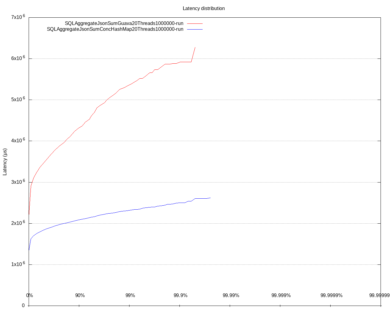
Let’s go straight to the flame graph of evaluation of a value from JSON:

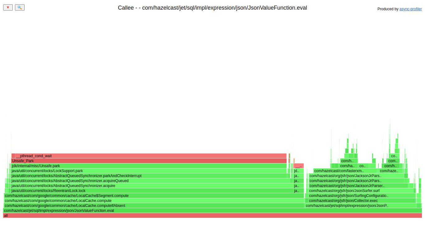
The big left part of that graph is acquiring a lock; it utilizes:

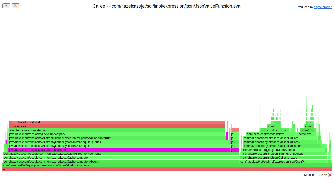
~70% of the time of evaluation of the value. That part of the code uses a Guava cache that uses ReentrantLock internally. The cache contains a mapping from the string JSON path to our object representing that path. The usage of that cache is usually single insert and multiple reads. For such a usage pattern, the ReentrantLock is not the best choice, ConcurrentHashMap is better, for example. A simple switch from Guava cache to CHM did this improvement:

In the end, we decided to do two implementations of a cache, one for a single JSON path based on a field, and the second for the rest of the cases.

The thing to remember is that the performance bottleneck may be in 3rd party libraries/frameworks. It doesn’t mean that their code is terrible. Usually we do not know the trade-offs there, and that may hurt us.

PR: https://github.com/hazelcast/hazelcast/pull/20655

Cluster side – scan for a single value by index

Benchmark details:

• Query: SELECT __key, this FROM iMap where col=...; // Index on col
• Values in IMap have two fields: String and int[20], serialized with IdentifiedDataSerializable
• IMap size – 10_000_000 entries
• Latency test – 7500 queries per second

This is a benchmark where we test a distributed deployment overhead of a job on a busy cluster. The part after the deployment is easy; we just need to take an index and fetch a single row from it. Unfortunately, in such queries, we will never be better than Predicate API since the execution plan for SQL is much bigger than for Predicate API, and serialization and deployment takes more time. What we can do is to speed up that part in SQL to be as fast as possible.

When I ran that benchmark’s first instance, the mean latency was around 4,5ms on a stressed cluster. To fight that kind of latency, we need to focus on all the resources that are required for that code to run. Let’s look at the heap allocation:

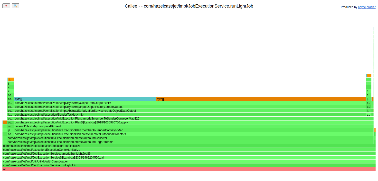
Over 90% of the recorded allocation (during the creation of the plan) was done in the constructor of SenderTasklet. That class is responsible for sending computation results to other nodes in the cluster. It created a 32k-byte array as a buffer of data to send. The value 32k was ok for a task manipulating multiple entries, but it was a waste of heap memory for a job that processes only one row.

We went with the solution to have a buffer with two initial sizes:

• Small initial size: 1k
• If that buffer is too small, it expands to 32k immediately

That approach didn’t hit larger tasks, they need to waste a 1k array at the beginning, but the allocation of such an array is much cheaper than 32k since 32k is often allocated outside the TLAB.

That change lowered the allocation rate of that benchmark from 3,8GB/s to 2,3GB/s, but that was not the only change in that part of our engine. My colleague pointed out that in some cases, we created a SenderTasklet that knew it would never send any data through the network. We can avoid the creation of unnecessary SenderTasklet. That change lowered the heap allocation rate to 1,5GB/s.

There were plenty of PRs for lowering that deployment overhead. The current status (mean) is:

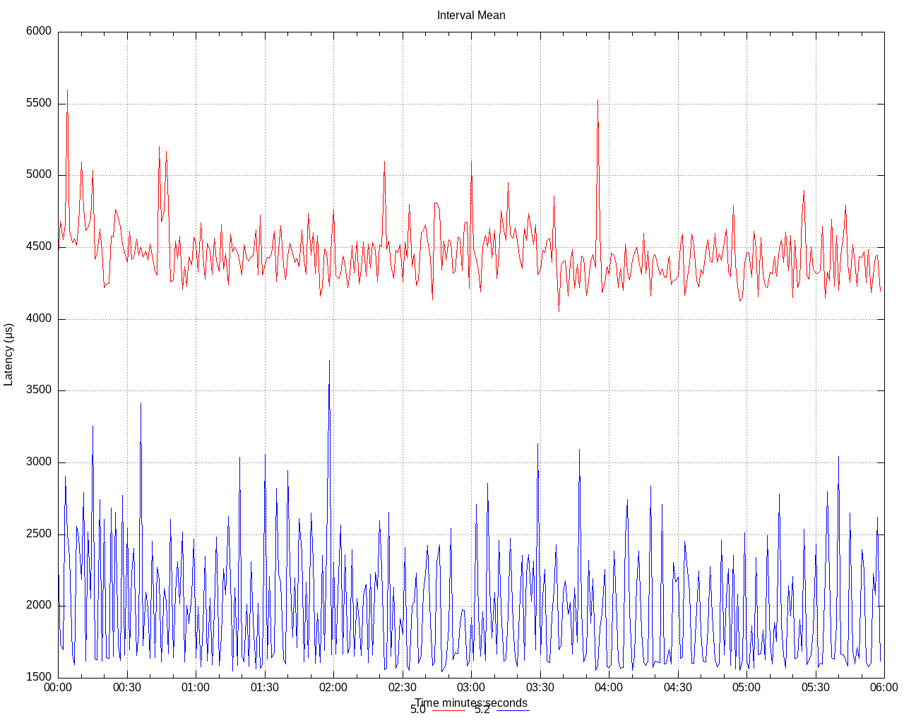
We lowered the mean latency from 4.5ms to 1.8ms on a stressed cluster, and we still have ideas for improving it.

The thing to remember is that allocation on the heap is fast, but no allocation is more immediate.

PRs: https://github.com/hazelcast/hazelcast/pull/20882 and https://github.com/hazelcast/hazelcast/pull/20940

Summary

Our SQL engine in release 5.2 is currently faster with better throughput than Predicate API in most of the benchmarks. The only kind of query where Predicate API is more immediate is a query that usually takes just milliseconds to execute. As I mentioned in the last example, we still have ideas on how to make the SQL engine faster. We are going to realize those in future releases.

In this post, I focused on four different issues that can teach us something. Let me gather those four things to remember:

• Performance is a living organism. It evolves with new features. What was efficient yesterday could be a bottleneck tomorrow.
• “If it looks stupid but works, it isn’t stupid” – every flame graph analysis technique is good as long as it works for you
• The performance bottleneck may be hidden in 3rd party libraries/frameworks
• Allocation on the heap is fast, but no allocation is faster

One additional “lesson learned” is that the Async-profiler is a handy tool for finding such high-level bottlenecks. You need to remember that there are issues in which such a profiler won’t help. Some performance bottlenecks can be understood after analyzing assembly code or with Top-down Microarchitecture Analysis.