Tracing a Single Operation in Distributed Systems

Let’s start with the basics. It is easy these days if we want to speed up a whole application! You run a JVM profiler, gather the results, and analyze the results to identify where the time and /or resources are wasted. Equipped with this understanding, you can make the application more efficient.

But what if we want to solve the problem of knowing why a single request is slow? It is tough to find a single request in profiler results. Additionally, as we will explore in this article, this problem becomes increasingly complex as we move from monolithic applications toward microservices, distributed architectures, and distributed systems.

Profiler mode

Often, the mistake made by software engineers during their initial profiling sessions is choosing the wrong profiler mode. Every profiler has multiple modes, and you need to select the one to help you solve your problem. The most common issues are:

• “my application/request is slow” – essentially, you want to measure where time is wasted; the correct mode to use is “wall-clock“
• “my application/request consumes too much CPU” – here, one would like to identify the section of code that is consuming excess CPU, and the “CPU” mode should be used
• “my application/request has a high allocation rate” – you should use “allocation” mode for this analysis

A common mistake is using “CPU” mode to analyze why an application is slow. If your application is CPU intensive, then yes, it may work. But if your application waits on IOs (like WS invocations or DB queries), locks, or waits, you will waste your time.

Since we want to solve the problem of slow requests, we’ll use the “wall-clock” profiler mode.

Profiler

Nowadays, we have plenty of profilers on the market. We need to select a profiler that supports “wall-clock” mode and runs with a small overhead so that it can even be used on a production system. The only profiler that fits these requirements that I am aware of is the Async-profiler, so we will focus on this one. It also supports dumping results in JFR format where each sample contains:

• Stacktrace
• Thread name
• Timestamp
• Thread state – if that thread consumes CPU or not

Monolithic application

Let’s start with a monolithic application’s most straightforward architecture to trace. A single thread processes the majority of the requests in a monolithic application. If we know the thread that has executed a slow request, then JFR output contains all the information we need. We need to filter that file with two filters:

• Thread name – it should equal the one that has processed the request
• Timestamp – it should be between the start and the end of the request execution

There are multiple ways of gathering this in our application. We can use our application log or application server access log.

Distributed architecture (like microservices)

The situation is more complicated in distributed computing architecture since one request is processed by multiple JVMs (we focus only on JVM applications here; this article will not solve problems in other execution engines). The standard approach to understanding what is happening in such an architecture is to use “correlation id” (in short, CID). The first application that receives a request from an outside world generates a CID passed in every request between applications in a distributed architecture—adding that CID to our logs, we can extract the specific thread on a particular JVM that executed the request. Then like before, we need to filter the JFR files from all the applications. It is exhausting but doable. We need to have the profiler running on all the JVMs.

Distributed systems

First of all, let’s understand the difference between distributed systems and distributed architecture. Those phrases are often used interchangeably, but the distributed systems I am referring to in this article are entirely different from distributed architecture. For this article, let’s assume that a distributed system is a single system in the architecture that distributes the work to multiple instances and threads to give the response ASAP.

You can imagine how difficult it is to trace a single request with such a definition. It is executed not only on multiple threads but also on multiple JVMs. How the hell can we trace that? Is that execution slow on each node? Or maybe one node is slower? Or maybe one thread on one node has too much work? How can we distinguish that?

The first approach is creating a CID and logging the thread on which JVM executes it. It would work, but it would be even more painful than the distributed architecture problem. To troubleshoot this problem regularly, well, we need something more innovative. What if we could add the CID to the JFR file? That would be great, as we wouldn’t have to aggregate multiple data sources. We would need the CID and JFR files from all the JVMs, and the only filter we need to apply to the JFR file is equality to CID.

Bad news

Well, Async-profiler has no such feature, so we have two options:

1. “roll over and die” and accept the current state of the reality and be miserable
2. or we can create our reality and software that fulfills our needs

As a software engineer, you have an opportunity no other profession has. You can choose option two! The easiest way to modify Async-profiler was simply by contributing to the open-sourced project. I prepared a PR: https://github.com/jvm-profiling-tools/async-profiler/pull/576. When writing this article, this PR had not been merged. It may never be merged, but the PR state is good enough to solve my current problem of finding the cause of long requests using the benchmarks on my test environment.

Good news

Even if my PR is not merged, the contextual profiling feature is on the Async-profiler roadmap; it will support this functionality sooner or later.

JFR filtering and transformation

We now have a tool that gathers the needed information in JFR format; great! Next, we need a tool that filters that output and presents it in a human-readable format. My favorite format to understand profiler output is a flame graph. Previously, I had written a tool that filters and converts JFR to flame graph, which I have now extended. It was straightforward as it’s just parsing, filtering, and transforming problems. That change is already in a master branch of my tool https://github.com/krzysztofslusarski/jvm-profiling-toolkit.

We have all the tools we need; let’s try it now!

Benchmark details:

• Hazelcast cluster size: 4 
• Machines with Intel Xeon CPU E5-2687W
• Heap size: 10 GB
• JDK17
• SQL query that is benchmarked: select count(*) from iMap 
• iMap size – 1 million java serialized objects
• Benchmark duration: 8 minutes 

The latency distribution for that benchmark:

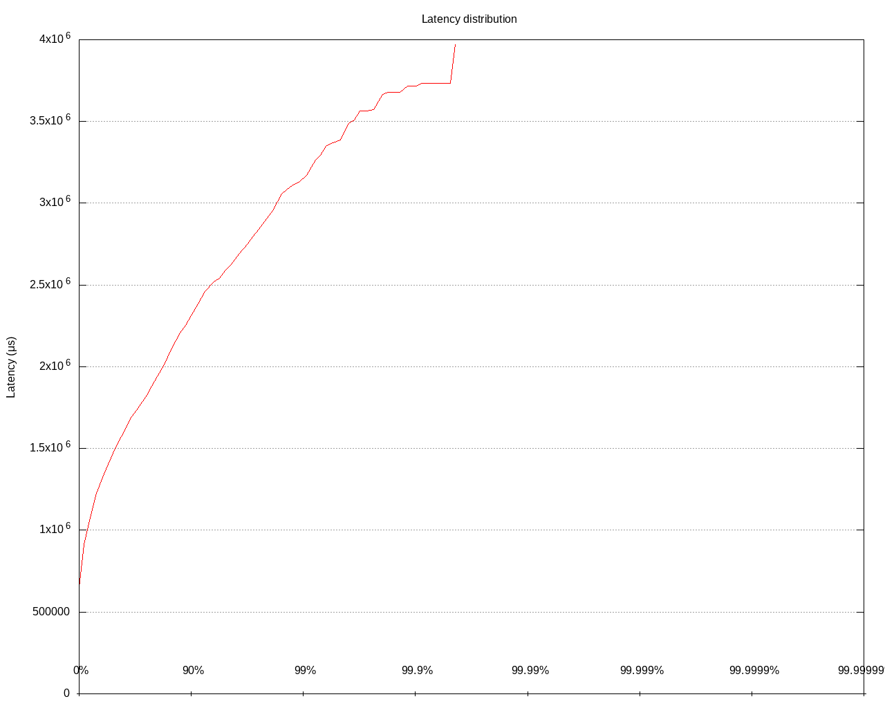
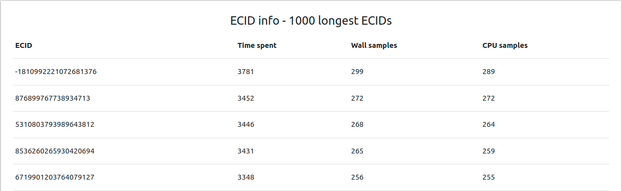
The 50th percentile is 1470 ms, whereas the 99.9th is 3718 ms. Let’s now analyze the JFR outputs with my tool. I’ve created a table with the longest CIDs in the files:

Let’s analyze a single CID. I selected additional levels in my tool, namely the filename and timestamp. The full flame graph:

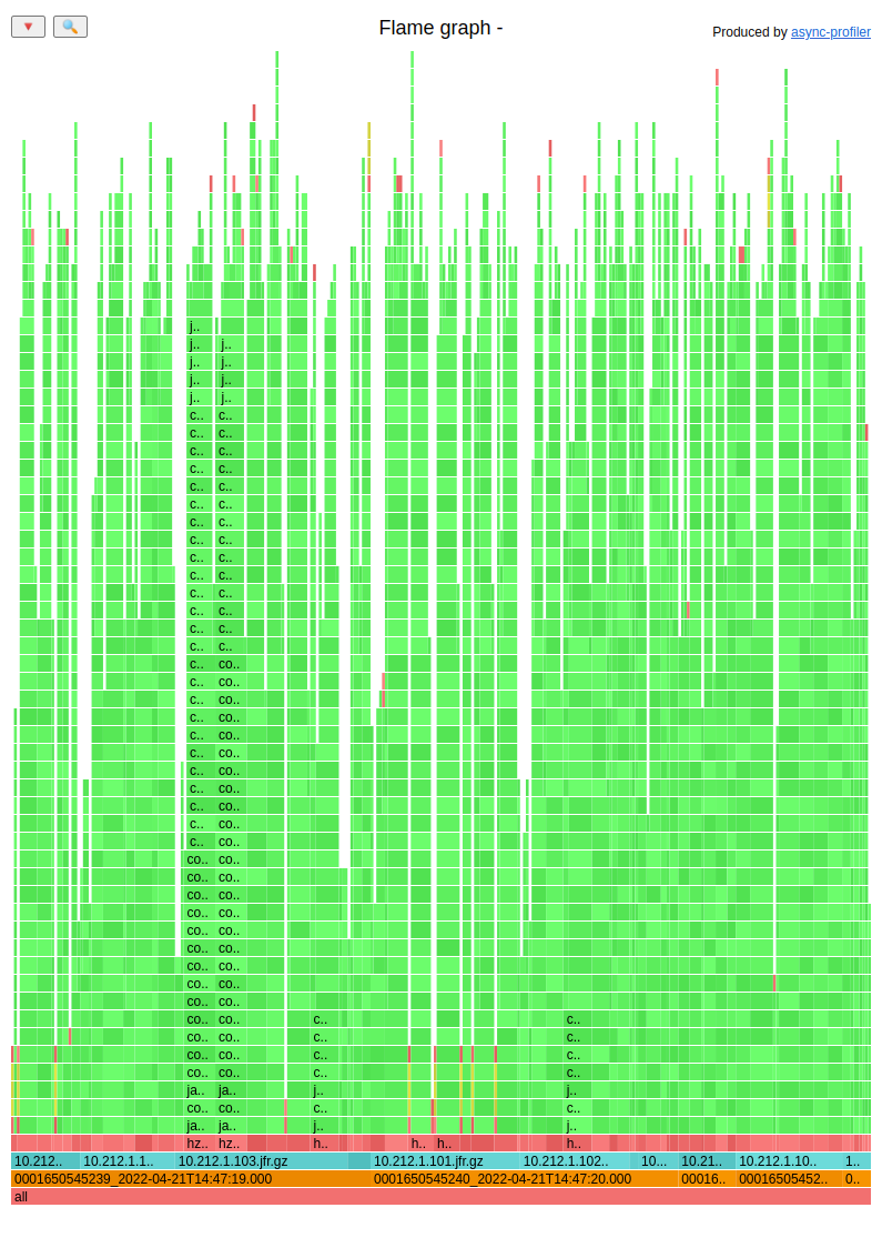
Let’s focus on the bottom rows:

The brown squares are timestamps with human-readable dates. The cyan ones are filenames from which upper stacktraces come.

Let’s start with timestamps and highlight them one by one:

Summing that up:

• 41.91% of samples were gathered between 14:47:19 and 14:47:20
• 35.79% of samples were gathered between 14:47:20 and 14:47:21
• 6.68%   of samples were gathered between 14:47:21 and 14:47:22
• 12.37% of samples were gathered between 14:47:22 and 14:47:23
• 3.34%   of samples were gathered between 14:47:23 and 14:47:24

Let’s highlight the filenames (which are named with the IP of the server) one by one:

A little summary:

• 25.42% of samples are from node 10.212.1.101
• 23,75% of samples are from node 10.212.1.102
• 21.07% of samples are from node 10.212.1.103
• 29.77% of samples are from node 10.212.1.104

Since brown bars are sorted alphabetically by timestamps, we can conclude that the 10.212.1.104 server was doing any work in the last seconds of processing.

So, the server with IP 10.212.1.104 is problematic. Maybe it is slower. Perhaps the work between nodes was distributed without proper balance, and this server had more work to do. Maybe there were some long GC pauses on that server. That topic is out of scope for this article, so I won’t dig into it here.

I checked five more long latency requests and the results were the same, confirming that the 10.212.1.104 server is the problem. I want to point out in this article that we now have a tool that gives us a great starting point for further investigation.

Some caveats

1. The current state of my PR to Async-profiler is “not merged.” The API can change, the whole solution may be completely different in the end. My implementation uses JNI calls when passing CID to the profiler; this may be problematic in some applications. The additional overhead for passing the CID was ~0,06% with the example above. Remember that in Hazelcast Jet, we need to give new CID very frequently since our green threads execute multiple fast tasklets. Based on this, you should consider that PR as POC for now (https://github.com/jvm-profiling-tools/async-profiler/pull/576)
2. The Async-profiler sampling interval is one sample every 10ms. This rate allows you to track latencies with hundreds of ms or more. With lower latencies, you need pieces to be gathered more often. The sampling interval can be changed, but it may degrade your performance if you sample too frequently.