Jet Calculates Pi Using Python

Today is PI DAY! Obviously, Pi has rather more than 2 decimal places. To have some fun, let’s use Jet to drive multiple Python workers to calculate Pi with increasing accuracy.

A tiny bit of mathematics

Pi is the ratio of a circle’s radius to its circumference. It’s 3.14. It’s 3.1416. It’s 3.14159266 or whatever. It has apparently an infinite number of decimal places.

But how to calculate it?

There are various ways, but here we’re going to use the “Monte Carlo method.”

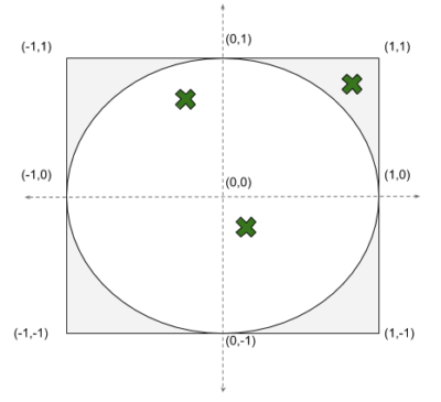
Picture a circle that exactly fits inside a square so it touches at the edges, as per the diagram. If we randomly generate points inside the square (the green crosses), some will be inside the circle and some won’t. The proportion of points inside compared to outside multiplied by 4 gives us an approximation to Pi. The more random points we generate, the better the approximation becomes.

Our circle has a radius of 1.0 and is centered on (0, 0).

We generate random points within the square where X varies randomly between -1 inclusive and +1 inclusive, and where Y varies randomly between -1 inclusive and +1 inclusive.

To calculate whether the generated (X, Y) coordinate is within the circle, all we need do is add X squared to Y squared and see if these two values added together are less than or equal to the radius squared. Conveniently, but not coincidentally, the radius is 1.

The Python code

Here’s the Python code:

for point in points:
      count_all += 1
      xy = point.split(',')
      x = xy[0]
      y = xy[1]
      x_squared = float(x) * float(x)
      y_squared = float(y) * float(y)
      xy_squared = (x_squared + y_squared)
      if xy_squared <= 1 :
        count_inside += 1

      pi = 4 * count_inside / count_all

It is keeping a running total of points inside the circle (“count_inside“) and all points (“count_all“).

Suppose the first point is (1, 1) which is outside of the circle. Using the running total of zero points inside we estimate Pi as 0.000000.

Imagine now the second point is (0, 0), which is inside the circle. Now, our running total is 1 point inside from 2, so we now estimate Pi as (4 * 1) / 2, or 2.000000.

Let’s use a third point (0.5, 0.5), which is also inside the circle. Our running total is 2 points inside from 3 and now we estimate Pi as (4 * 2) / 3, or 2.666666.

Finally, a fourth point (0.6, 0.6), again is inside the circle. The running total of 3 points inside from 4 gives an estimate for Pi of (4 * 3) / 4, or 3.000000.

Ok, so 3.000000 is still a poor estimate for Pi, but it’s better than the previous value 2.666666, which was better than the predecessor 2.000000 and certainly better than 0.000000.

That’s the theory in practice. With each new random input point, the estimate for Pi becomes more accurate.

Jet 4.0’s Python runner

Refer to the following diagram.

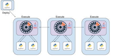
Python code is interpreted, meaning it’s just a collection of files or even more simply can be viewed as a string. Very easy to deploy.

In the diagram, the Python code module is on a host machine in the top left corner. The deploy process streams this Python code from the host machine in the top left corner to one of the Jet host machines in the lower half of the diagram, which in turn duplicates the deployment across all Jet machines.

When the job using the code runs, each Jet instance (a JVM) runs one or more Python virtual machines on that host. Here there are three Jet instances and each of these spins up two Python workers with data passing in and out via open GRPC sockets. So, here we actually have six running Python workers passing data back and forwards with three Jet instances. Hopefully, the Python workers are stable and won’t crash, but if they do Jet won’t fail.

localParallelism

When Jet runs a Python worker in a pipeline stage, there is an optional parameter localParallelism.

This controls how many Python workers will run for each Hazelcast Jet node and will – by default – be derived from the number of CPUs, one worker for each.

In other words, Jet will launch multiple Python workers for the job to maximize usage of the available CPUs and hence processing capacity. Input will be striped by Jet across the available workers.

requirements.txt

Python is an interpreted language and may make reference to libraries such as numpy and pandas.

In standard Python fashion, these libraries should be listed in a requirements.txt file, which Jet will download before executing the Python job.

For faster job start-up, you can pre-install the requirements to the hosts running Hazelcast using pip3. In a Docker environment, you should build these into your Docker image.

First attempt

Here’s the first attempt as a Jet pipeline to calculate Pi.

Input

A custom input source has been defined, which generates an infinite stream of (X, Y) coordinates into a map.

The code for this is essentially this:

void fillBufferFn(SourceBuilder.SourceBuffer<Map.Entry> buffer) {
    Tuple2 tuple2 = Tuple2.tuple2(random.nextDouble(), random.nextDouble());
    buffer.add(tuple2);

A Tuple2 is a Jet convenience class to hold a data pair. There is also Tuple3 for a trio of data items. Tuple4 for four data items together.

So a Tuple2 is a map entry, where X is the entry’s key and Y is the entry’s value. We use the map as the input source for our pipeline.

This generates an unlimited number of points, which is what we need for our estimation calculation to become more accurate. However, we need eviction on the target map so we don’t run out of storage space.

Pipeline

We already shared the Python code above. Now, let’s see how Jet runs it.

pipeline
.readFrom(Sources.mapJournal("points", JournalInitialPosition.START_FROM_CURRENT)).withIngestionTimestamps()
.map(entry -> entry.getKey() + "," + entry.getValue())
.apply(PythonTransforms.mapUsingPython(getPythonServiceConfig("pi1")))
.window(WindowDefinition.tumbling(TimeUnit.SECONDS.toMillis(5)))
.aggregate(AggregateOperations.averagingDouble(string -> Double.parseDouble(string)))
.writeTo(MyUtils.buildTopicSink(Pi1Job.class, "pi"));

We define a pipeline that reads from a Map.Entry holding our (X, Y) coordinates. We reformat this as a CSV separated string and pass it into a Python script with the given name.

From the answer that the Python workers give us, we calculate the average of these every 5 seconds and publish this to a topic named “pi“.

Easy!

Visualization

This diagram tries to visualize what is happening:

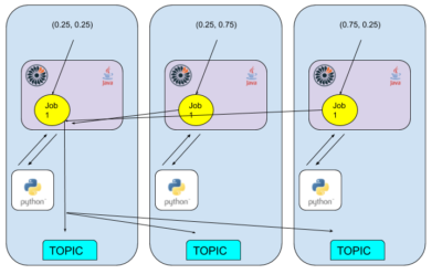
Here we imagine there might be three nodes, each running one Jet instance.

Each is generating X and Y randomly and in parallel, but these points are passed into the Jet job named “Job 1“.

“Job 1” takes this input locally (ie. for each Jet instance), and passes it into local Python workers. For simplicity, we assume one Python worker per Jet node — more Python workers are better for performance but will make the diagram too complicated.

The Pi value calculated by each Python worker is aggregated/collated on one of the Jet nodes (let’s assume the one of the left) and then broadcast to a topic which is available on all nodes.

Output

The pipeline outputs the result every 5 seconds.

***************************************************************    
Topic 'pi' : Job 'Pi1Job' : Value '3.145907828268894'        
***************************************************************    

So what’s wrong with this?

This approach is not mathematically correct, though you’re a good mathematician if you’ve spotted it before reading this section.

Each Python worker calculates Pi independently and the average is taken. However, the average of the sum of quotients is not equivalent to the quotient of the sum.

Imagine three Python workers and a sequence of four input points, the first three of which lie within the circle.

Two Python workers receive an input point within the circle, each estimates Pi as (4 * 1) / 1, or 4.000000.

One Python worker receives an input point inside and an input point outside the circle, estimating Pi as (4 * 1) / 2, or 2.000000.

The average of the three Python’s workers estimates is (4.000000 + 4.000000 + 2.000000) / 3, or 3.333333. However, for the actual input, the right answer is (4 * 3) / 4, or 3.000000.

The business logic is wrong, it wouldn’t be the first time. Won’t be the last time either.

The code is stateful

The Python code keeps running totals here

count_all += 1

and here

count_inside += 1

for the points processed and number inside the circle.

This is local to the Python worker and not saved anywhere. If the Python worker is restarted, its running totals are lost and begin again from zero.

Jet will stop the Python workers while the cluster changes size (Hazelcast nodes join or leave) and restart them with the input load re-partitioned across the new cluster member nodes.

Second attempt

The first approach is not right. Let’s try again.

Input

The input for this attempt is the same as the input for the first attempt.

We can only meaningfully compare the output from the first and second attempts if they are processing the same stream of random points. If they had different streams of random points, the comparison would be weakened.

Python code

The Python code is slightly amended from the first attempt.

from tribool import Tribool

def handle(points):
    results = []

    for point in points:
      xy = point.split(',')
      x = xy[0]
      y = xy[1]
      x_squared = float(x) * float(x)
      y_squared = float(y) * float(y)
      xy_squared = (x_squared + y_squared)
      if xy_squared <= 1 :
        result = Tribool(True) 
      else :
        result = Tribool(False) 

Now all we output for each input point is “true” or “false” for whether the input point is inside the circle or not. We don’t keep running totals in the Python worker anymore.

Note also, just for fun “from tribool import Tribool” to import an optional library.

Pipeline

Finally, we have amended the Jet pipeline so that Jet (in Java) maintains the counts of points inside and outside the circle globally from all Python workers concurrently.

pipeline
.readFrom(Sources.mapJournal("points", JournalInitialPosition.START_FROM_CURRENT)).withIngestionTimestamps()
.map(entry -> entry.getKey() + "," + entry.getValue())
.apply(PythonTransforms.mapUsingPython(getPythonServiceConfig("pi2")))
.mapStateful(MutableReference::new, PI_CALCULATOR)
.window(WindowDefinition.tumbling(TimeUnit.SECONDS.toMillis(5)))
.aggregate(lastInWindow(Double::doubleValue))
.writeTo(MyUtils.buildTopicSink(Pi2Job.class, "pi"));

For the pipeline, it’s the same start, but what comes out of Python now passes through this:

BiFunctionEx<MutableReference<Tuple2>, String, Double> PI_CALCULATOR =
    (MutableReference<Tuple2> reference, String string) -> {
        long trueCount = 0;
        long falseCount = 0;

        Tuple2 previous = reference.get();
        if (previous != null) {
            trueCount = previous.f0();
            falseCount = previous.f1();
        }

        if (string.toLowerCase().equals("true")) {
            trueCount++;
        } else {
            falseCount++;
        }

        Tuple2 next = Tuple2.tuple2(trueCount, falseCount);
        reference.set(next);

        return 4 * trueCount / (trueCount + falseCount);
    };

Now a Jet job stage is keeping the running totals and everything comes out in a five second window to a topic as before.

This is mathematically better but pushes some of the calculation into the pipeline. That’s not exactly a bother but it does make it a little harder from a support perspective to work out what is happening where in terms of the calculation.

Visualization

Now let’s try this diagram:

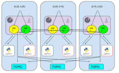
We have added a second job, named with great imagination “Job 2“.

“Job 2” takes the same input source as “Job 1” and again runs in parallel across the Jet nodes. This time, “Job 2” sends its input to different Python workers to calculate Pi, collates on one of the Jet nodes (the right one this time), and publishes to a topic across all nodes.

The diagram now looks a little cluttered. “Job 1” is running across all Jet nodes, running one version of the Python code in Python workers. “Job 2” has been added, also running across all Jet nodes, running a different version of the Python code in different Python workers.

So, in effect, we have two different Python programs, processing the same input source and putting output to the same output sink.

Output

The pipeline outputs the result every five seconds, the job name has changed and obviously the derivation of Pi is different so the output will have varied from the first attempt most likely.

***************************************************************    
Topic 'pi' : Job 'Pi2Job' : Value '3.1585789532668387'      
***************************************************************    

Is the second attempt better than the first attempt?

The second attempt is mathematically correct so theoretically is best. But the business logic is in two places, in Python code and Java code, which makes it harder to follow.

Given enough input, the first attempt will produce a reasonable approximation to Pi, so perhaps it is good enough. Simplicity could be a preference over absolute correctness.

Two attempts at once

What’s crucial to note here is that you can run both attempts concurrently.

Jet runs each job in a sandbox (or in Java terms, a classloader).

If you have a new version of your processing logic, you can stop the old one and start the new one. That’s a simple approach, and in many ways appealing. However, for some period neither is running and if your job is doing something business-critical that’s no good.

With Jet, you can run both jobs concurrently from the same input. You need some way to distinguish the output in order to decide if the new version is an improvement (here it’s just a publish to a topic with the job variant name). Once you have decided, you can shut down the whichever is performing the worst.

This is a clear improvement in terms of no loss of service, but you have to note that adding an extra job increases the processing load. If your processing time is critical, you should consider temporarily scaling up the cluster size to accommodate the dual processing of some input.

Summary

Jet can run Python workers in a pipeline, streaming or batching data into them, spinning up multiple Python workers automatically and adjusting when nodes join or leave the cluster.

All you need to provide Jet with is the location of a Python script. Jet will push it to all nodes in the cluster and run it concurrently for you.

If you want to try this yourself, the code is here.

The Python code here is just a trivial example, but it can be anything, including Machine Learning of course.