Where Are My Keys ?

It’s useful to understand how, why and where Hazelcast stores your data in the grid.

What happens is what you really need, but it won’t necessarily be what you first think you want.

We’ll explore this in this blog by putting some number keys in a map, a common starting point and source of confusion.

A Map

A “map” is a data structure in Computer Science that is sometimes called a key-value store or a “dictionary.” Here’s one way to think of it:

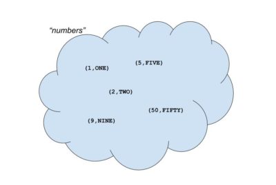
Our map here is some sort of logical collection of data pairs. We’ve named it “numbers” to distinguish it from other data collections we may have. It contains some but not all numbers, and there’s no implication that these are stored in any particular order.

Five data records are shown. The left side of the entry record is the key, here a number. The right side of the entry record is the value, here a string.

The keys are unique. Values don’t have to be unique. Though it makes sense for this example.

It’s similar to looking up a word in a real dictionary. We have a word key we wish to lookup. This is used to find and return the corresponding definition.

It’s also a bit like “SELECT * FROM table WHERE primaryKey = $1” in SQL terms.

Our data record has a primary key. We wish to retrieve using the primary key. This is what a map does best.

IMap

IMap is Hazelcast’s implementation of the classic map data structure.

In a Hazelcast data grid, there are usually several nodes doing data storage.

In this case, the IMap would be spread across these processes. Each process hosts a share of the map’s contents.

This gives the obvious benefit of scalability. With three nodes, each node hosts a third of the map. So the map’s capacity is triple the capacity of a single process. If we add a fourth process, the map’s capacity is now four times that of a single process. We have scaled up.

However, there is also the potential for confusion if you don’t understand some of the necessary implementation details.

For example, with 3 processes, each has ⅓ of the map to look after but it might not mean ⅓ of the data.

⅓ Map != ⅓ Data

Our “numbers” map if stored in Hazelcast might look like the below:

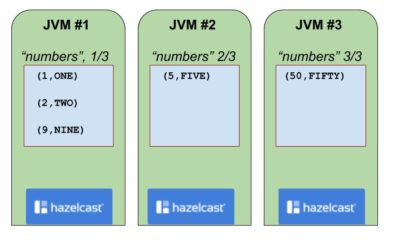
One JVM process has 3 data records. The other two have 1 data record each.

Counter-Intuitive

So, here is the first counter-intuitive point.

It seems reasonable enough that 5 data records split across 3 processes doesn’t result in 2.666 records each. Hazelcast does not break an individual data record.

However, 2, 2 and 1 would surely be a more even spread of records than 3, 1 and 1 ?

Yes, it would. So we need to look deeper to understand.

Partitioning

We don’t just want to store data in Hazelcast, we want to get it back out again, and quickly.

So how is this done?

In a real physical dictionary, an actual book, if we wanted to find the definition for the word “Hazelcast” we would not start at the first word (“aardvark”?) and scan forward. The dictionary is ordered into sections, so we would jump to the “H” section for words beginning with “H*” and look from there.

Hazelcast takes a similar approach. The map is divided into logical sections known as partitions, based on the system property hazelcast.partition.count and we have an algorithm that dictates which partition holds any particular key.

The default value for “hazelcast.partition.count” is 271.

A dictionary for English words might use 26 partitions, as there are 26 letters in the English alphabet.

Hazelcast is capable of storing more than just words. Here it is doing numbers. So we still need to understand why 271 is used.

Partition Allocation

When a map is first created, it is empty obviously, as no data can have been inserted.

However, at this point, the 271 partitions will be allocated to the storage members of the cluster. They are allocated as evenly as can be and with a degree of randomization.

We can never know in advance what keys might be inserted, but if we’ve spread out the partitions on the available members, we’re as ready as we can be.

Key to Partition Algorithm

So all we need know is where the partitions are, and we quickly find any one key by looking in exactly one partition.

A common supposition is that key placement should be round-robin. With 271 partitions we might expect key 1 to go to partition 1, key 2 to partition 2, key 3 to partition 3 and so on up to key 271 where we go back to partition 1 and repeat the loop.

In fact, the algorithm is only slightly different, to work around two flaws in this approach.

The first flaw is obvious, not all keys are numbers. Keys can be strings, UUIDs, or even images. Anything so long as they can be transferred across the network.

The second flaw is more subtle and insidious, keys may have patterns in their allocation. If our keys were the sequence 29, 300, 571, 842, 1113 and 1384 we might think them to be random, but in fact the change from key to key is the same. If this change lines up with the partition count, then a round-robin approach would see all keys end up in the same partition.

Key to Hash Code

So, how do we find the partition for the key in the real world to avoid the pitfall that the key may not be numeric and keys may have echelon patterns?

The solution is to use a hashing function, which will take any type of object and return a number. While the output number is not required to be unique (two keys can hash to the same value), we wish the range of output values to be evenly spread even if the range of input values is uneven.

Java provides a “hashCode()” function for objects, which most IDEs will generate for you. This is not used. Partly because Hazelcast is used by non-Java code such as .NET and Python. And partly also because it doesn’t produce a particularly good spread of output values.

Instead, we use the “murmur hash 3” algorithm, which is described here and in many other places.

Murmur Hash 3

Hazelcast’s implementation of Murmur Hash 3 is here for Java, and with matching implementations for each of the client languages.

The murmur algorithm is fairly complicated mathematics, with bit shifting and binary arithmetic. If you’re interested in going further, please follow the Wikipedia link to learn more. And if not, just regard it as a trusted function that gives the desired output.

Why 271

The final piece of this little puzzle is why 271.

What is significant about 271 in this context is it is a prime number.

We take the modulus of the hash output by the partition count to determine the partition. Although the hash function should give us a spread of output values for uneven input, using a prime number for the modulus further enhances this even data spread.

For example, if the key is 1 the hash code might be 768969306. If we do 768969306 % 271, the modulus or remainder is 31. So integer key 1 belongs in partition 31. Partition 31 may not have that key, because it may not have been written, but we know the only and only partition to look in to confirm.

Checkpoint

So now we have an explanation.

Code below will show that the keys 1, 2, 5, 9 and 50 are assigned to
partitions 31, 5, 169, 42 and 105 respectively.

In our 3-nodes cluster, the 271 partitions mean the nodes get 90 or 91 partitions each, the best we can spread them out. Recall that when we do this, we don’t know what data will be inserted.

At this point, it’s not unreasonable that the node on the left of the diagram above owns partitions 5, 31 and 42, along with nearly ninety other partitions.

In fact, if we only inserted records with keys 1, 2 and 9, we would find all our data on one node.

And this really is ok. The partitioning scheme is designed to spread the data when we have millions or billions of data records.

If we have a trivially small number of records, such as the three or five here, we need to expect this apparent imbalance. With very small numbers of records, the actual imbalance should be negligible for small records. Should it ever become problematic, a Near Cache is the answer.

Show Me the Code

The code for this example is available here.

What it does is create a 3-node cluster and inject integer keys from the range of 0 to 24.

It implements a simplified version of the Murmur 3 algorithm, specifically for integers which we know to be four bytes, to determine the hash code value and expected partition for each key. Hazelcast has a function `instance.getPartitionService().getPartition(K)` which will actually tell us the partition that Hazelcast would select for our key, so we use this to compare our predicted partition with the actual.

So, we can predict and verify which partition will host our key. We can’t predict which Hazelcast member will host that partition, as this is non-deterministic. However, we can ask Hazelcast.

So there is a call to `ExecutorService.submitToKeyOwner(callable, K)` where we request a callable run on the node that owns the given key. This callable returns the node name, so we find out which node in the cluster is hosting which key.

Code Output

If we run the example it creates a 3-node cluster and we see output like

Key '1', hashcode 768969306, is in partition 31, hosted currently by node node0
Key '2', hashcode 832990049, is in partition 5, hosted currently by node node0

Integer key 1 has a hash code of 768969306. The modulus of 768969306 % 271 is 31. So integer key 1 is in partition 31. This is on node 0 of the 3-node cluster.

Key 2 has a hash code 832990049. If we do 832990049 % 271 we get 5. Key 2 is in partition 5. This is also on node 0.

Both keys 1 and 2 are on the same node because that one node is responsible for the two partitions relevant.

Now let’s run the example again:

Key '1', hashcode 768969306, is in partition 31, hosted currently by node node1
Key '2', hashcode 832990049, is in partition 5, hosted currently by node node0

This creates a fresh 3-node cluster. The output is similar but not identical.

The calculated hash codes for keys 1 and 2 are the same, and therefore so are their partitions. Hashing must be deterministic.

Partition allocation is not deterministic. In the second run, a different node is responsible for partition 31 compared to partition 5, so the keys are on different nodes now.

One last point to look at here is keys 15 and 16.

Key '15', hashcode 1398412787, is in partition 213, hosted currently by node node1
Key '16', hashcode 1099026892, is in partition 213, hosted currently by node node1

They have different hash codes. When the hash code has modulus 271 applied, keys will end up sharing partitions as we have more keys than partitions. Sometimes this will be consecutive keys.

Since keys 15 and 16 are in the same partition, they will always be on the same node, regardless of the cluster size.

Checkpoint

As` a bonus, there is one last problem.

In the code,

for (int i = 0 ; i < 25 ; i++) {
    ....
    byte[] value = new byte[i];
    iMap.set(i,  value);
}

We are iterating through the keys, but the value associated gets bigger. For key 1 the value is 1 byte, for key 2 the value is 2 bytes, and so on. The value for key 25 is 25 bytes, 25 times more than for key 1.

Even if we had 25 Hazelcast servers and it happened that they had 1 of the 25 keys each, there would still be an imbalance as the data records are not the same size.

Normally you would expect variable-sized records to vary within a range rather than continually get larger, but this is a feature of the application. Hazelcast stores what it is given.

Summary

The use of prime numbers and hashing algorithms make it reasonably likely that a Hazelcast cluster will remain balanced for large data volumes.

It is however not a guarantee.

When having strange patterns to key allocation, it is possible that data allocation might not be uniform. Some partitions may get more records than others.

Equally, if data records are of variable size, wild variations can always result in an uneven spread of data. Partitions may have the same number of records but if the records are different sizes the partitions will use different amounts of memory.

So it’s worth keeping an eye on the monitoring, the counts of the number of entries per member and the total size of each member.