
Principal Architect
With over 30 years of industry experience, Neil has designed, developed, debugged, and supported software systems for numerous customers large and small. Initially, a C and assembler programmer, most of the last 20 years have been Java-based, with a focus on distributed systems, data grids, and stream processing. Neil is an occasional committer to the Hazelcast code base, with special interest on GoLang.
View all blogs by the authorMay 2, 2019
Calculation in Hazelcast Cloud
This is an example showing one way you might connect to Hazelcast Cloud, and how you can harness its power for improved performance.
As a problem, we’re going to calculate the spread of customer satisfaction, as the average doesn’t give enough insight.
The example shows a custom domain model and server-side code execution. It shows both the junior and senior developer approach to cloud computing, with the latter being substantially more efficient.
The problem
For this example, we’re going to do a statistical calculation known as Standard Deviation.
Don’t worry, the math here is straightforward and there are no Greek letters or fancy symbols. If you already know how this calculation works you can skip the following subsection.
Standard Deviation explained
One thing we are often interested in is averages.
For the numbers 1, 2, 3, 4 and 5 the average is 3.
For the numbers 2, 2, 3, 4 and 4 the average is also 3.
And for the numbers 1, 1, 3, 5 and 5 the average is again 3.
Hopefully, all clear so far!
There are five numbers in each group, the total for each group is fifteen, but the actual numbers differ.
One of the things we’d like to do is produce a simple metric for how much of a spread in the numbers there is.
In the second group (2, 2, 3, 4 and 4) most of the numbers are one away from the average of 3. In the third group (1, 1, 3, 5 and 5) most of the numbers are two away from the average.
There are lots of ways to do this. Lots. The “standard deviation” here is just a name that means it has been adopted as a standard for calculating how numbers deviate from the average.
How it works is for each number we calculate how much this differs from the average. This difference is squared and added to a running total.
Once we have this total, we take the average of this. So now we have the typical square of the difference from the original average.
Finally, we take the square root of this, to result in a single value that we call the standard deviation.
The first set of numbers
Let’s do this calculation for the numbers 1, 2, 3, 4 and 5, which we already know has the average of 3.
- The difference between the first number (1) and the average (3) is 2. Squaring this gives 4 which starts the running total at 4.
- The difference between the second number (2) and the average (3) is 1. Squaring this gives 1, adding to the running total takes this running total to 5.
- The difference between the third number (3) and the average (3) is 0. Squaring this gives 0, so the running total stays as 5.
- The difference between the fourth number (4) and the average (3) is 1. Squaring this gives 1, taking the running total to 6.
- The difference between the last number (5) and the average (3) is 2. Squaring this is 4, taking the running total to 10.
- The running total is 10 and there were 5 numbers, so the typical square is 10 divided by 5, that is 2.
- The square root of 2 gives us a standard deviation of 1.41.
The second set of numbers
This sort of calculation is a bit tedious, which is why we want the machines to do it. But as we’re enthusiastic, let’s do this again for the numbers 1, 1, 3, 5 and 5, and their average of 3.
- The first number (1) differs by 2 from the average. Squaring 2 starts the running total with 4.
- The second number (1) also differs by 2 from the average. Squaring 2 gives 4, taking the running total to 8.
- The third number (3) is the same as the average, so the square is 0 and the running total stays as 8.
- The fourth number (5) differs by 2 from the average. Squaring 2 gives 4, taking the running total to 12.
- The fifth number (5) again differs by 2 from the average. This adds another 4 to the running total, taking it to 16.
- The running total is 16 for the 5 numbers, so the typical square is 16 / 5 = 3.2
- The square root of 3.2 we all know is 1.78 which is our result.
The answers
So where we end up is the standard deviation of the numbers 1, 2, 3, 4 and 5 is 1.41. The standard deviation of the numbers 1, 1, 3, 5 and 5 is 1.78.
The standard deviation of 1.41 for the one group being lower than the standard deviation of 1.78 for the other group gives us a simple metric that proves the first group of numbers doesn’t vary as much as the second.
The business logic
There are not many steps to business logic.
The first is to calculate the average of the input numbers.
The second is to calculate the running total of the square of how each number differs from the average.
The third is to calculate the average of the running total.
And finally, we take the square root of that and call it the standard deviation.
The optional magic
The optional magic is parallelism.
In the second step, we perform a calculation on each number. We take the difference for that number from the average and then square it.
This is open to parallelism. If we have more than one CPU we could run the “square of the difference” step for several numbers at once. All we need is a way to combine these independent answers into the running total.
This is where we’ll use Hazelcast Cloud.
We could do a similar thing in the first step too, but as it turns out, we have another trick to make that even simpler.
Test data
We shall stick with the five numbers 1, 2, 3, 4 and 5 since we have above the manual calculation of standard deviation resulting in 1.41.
To make it more realistic, we’ll make these numbers the “satisfaction” rating from some customers in this domain object:
class Customer implements Serializable {
    private String firstName;
    private int satisfaction;
So here what we are looking at is customer satisfaction. The average satisfaction is useful. To know the amount of spread between very satisfied and very dissatisfied customers is even more helpful.
Step 1 – The “Junior Developer” way
In the class “JuniorDeveloper.java“, the average is calculated like this:
int count = 0;
double total = 0;

for (Integer key : iMap.keySet()) {
    count++;
    total += iMap.get(key).getSatisfaction();
}

return (total / count);
This is pretty easy code to understand, so that’s a win from a maintenance aspect. However, it has three flaws.
The main one is performance. This code requires every customer record to be moved from where the data is stored (in this case Hazelcast) to where the calculation is run. Even if a projection were included, this is very heavy on the network.
There is a second issue. The “keySet()” operation produces a collection containing all the keys to iterate across. If this collection is huge, it could overflow the memory.
Lastly, there’s a division by zero if map is empty. A good unit test would find this.
Note: Let’s not forget maintenance. This code is easy to understand.
Step 1 – The “Senior Developer” way
In the class “SeniorDeveloper.java“, the average is calculated in one line:
return iMap.aggregate(Aggregators.integerAvg("satisfaction"));
Hazelcast provides in-built functions for typical calculations, so why not use them?
Senior developers do more thinking and less typing.
Hazelcast’s implementation is the same as the coding for senior developers in step 2. There are some internal optimisations so you won’t be able to beat it with your coding.
Note: Let’s never forget maintenance. Even if you don’t know Hazelcast, it’s relatively intuitive what is happening.
Step 2 – The “Junior Developer” way
In “JuniorDeveloper.java“, the sum of the square of the differences is calculated as:
double total = 0;

for (Integer key : iMap.keySet()) {
    int satisfaction = iMap.get(key).getSatisfaction();
    double difference = satisfaction - average;
    total += difference * difference;
}

return total;
This is not much different from the junior developer’s approach to step 1. The coding is pretty clear. Lots of data is retrieved. The “keySet()” operation may still overflow memory.
At least we don’t have to worry about division by zero. Unit tests will pass.
Note: Maintenance! So from a maintenance perspective, this is better — less faults than the junior developer’s approach to step 1 and very clear.
Step 2 – The “Senior Developer” way
This is where the magic starts to happen.
In Hazelcast, we can submit a Java “Runnable” or “Callable” task to run on the grid. We can select to run this task on one, some or all of the grid servers. So that’s what we do here.
The client uses Hazelcast’s ExecutorService to run a “Callable” on each grid server.
The callable itself is imaginatively named “TotalDifferenceSquaredCallable.java” and it runs this calculation on the Hazelcast server where it is invoked.
double total = 0;

for (Integer key : iMap.localKeySet()) {
    int satisfaction = iMap.get(key).getSatisfaction();
    double difference = satisfaction - this.average;
    total += difference * difference;
}

return total;
This is more or less the same calculation as in “JuniorDeveloper.java“‘s “totalDifferenceSquared()” method. We could add a stream or a lambda, but it wouldn’t be any different.
Where it is different is in three ways.
- Firstly, this calculation is parallelised. The Hazelcast client on your machine does this:
Map<Member, Future> results =
    executorService.submitToAllMembers(totalDifferenceSquaredCallable);
The task is sent to all grid servers in parallel.
Each server calculates a subtotal only for the data that server hosts. If you have two servers, the calculation takes half the time. If you have ten servers, the calculation takes a tenth of the time. Each server runs its calculation independently. The run time is dependent on how much data each server hosts rather than how much data as a whole exists.
- Secondly, to do this, the task uses the “
localKeySet()” method instead of the “keySet()” method. This method returns the keys that are held by the current process. And since we run the task on all processes, we cover all the keys. This makes a big difference.We are only looking at the keys, and therefore entries, hosted by the current process. So we don’t have to do any network call to retrieve them from elsewhere.And of course, the “localKeySet()” operation is asking for only the keys from an “EntrySet” hosted in local memory. The local “KeySet” must be smaller than the local “EntrySet” since we are ignoring the values so we should be less concerned about overflowing memory. The local “KeySet” returns a defensive copy of the “EntrySet” so it is not impossible. - Finally, the task is submitted across every member in the cluster, which gives us a collection of “
Future” objects to manage (“Map<Member, Future> results“). There is one “Future” for each member running the task, and we need to wait for them all to finish. This is not exactly difficult. Since all members will have roughly the same amount of data, we can assume execution time is equal. We can iterate across this collection running “Future.get()” to obtain the sub-total from each member.
Note: Maintenance, one more time. And this is a tough one. This coding has some obvious bits, but some other parts need a bit of Hazelcast knowledge. Is the performance boost worth the cost of understanding?
Run time complexity
So what is the difference between the two ways?
There are 5 data records, and the simplest Hazelcast cluster has one server.
The clever way requires five integers to be retrieved for the “satisfaction” field to run into the calculation. For simplicity, we obtain the whole data record for each.
The smart way runs the calculation on the one server and returns one double across the network.
So the choice is five network transfers or one. One is obviously less than five but does this matter?
Now imagine there are 1,000,000 data records and we chose to have 2 Hazelcast servers. One Hazelcast server could handle this volume but wouldn’t be resilient to failure.
So the simple way now retrieves 1,000,000 integers across the network and the clever way retrieves two doubles (one from each server).
It’s pretty clear that if data volumes scale, the server-side computation copes better. The same amount of data still has to be examined, but less data moves.
Do not forget concurrency
The coding in this example disregards concurrency. Generally, a bad idea unless you know what you are doing.
Step 1 calculates the average, then Step 2 calculates the deviation from the average.
It is possible that records are added or removed between steps 1 and 2, which makes the calculation wrong.
While there are ways to deal with changing data, here it is almost axiomatic that the data cannot change when an average calculation is being used.
Running the example
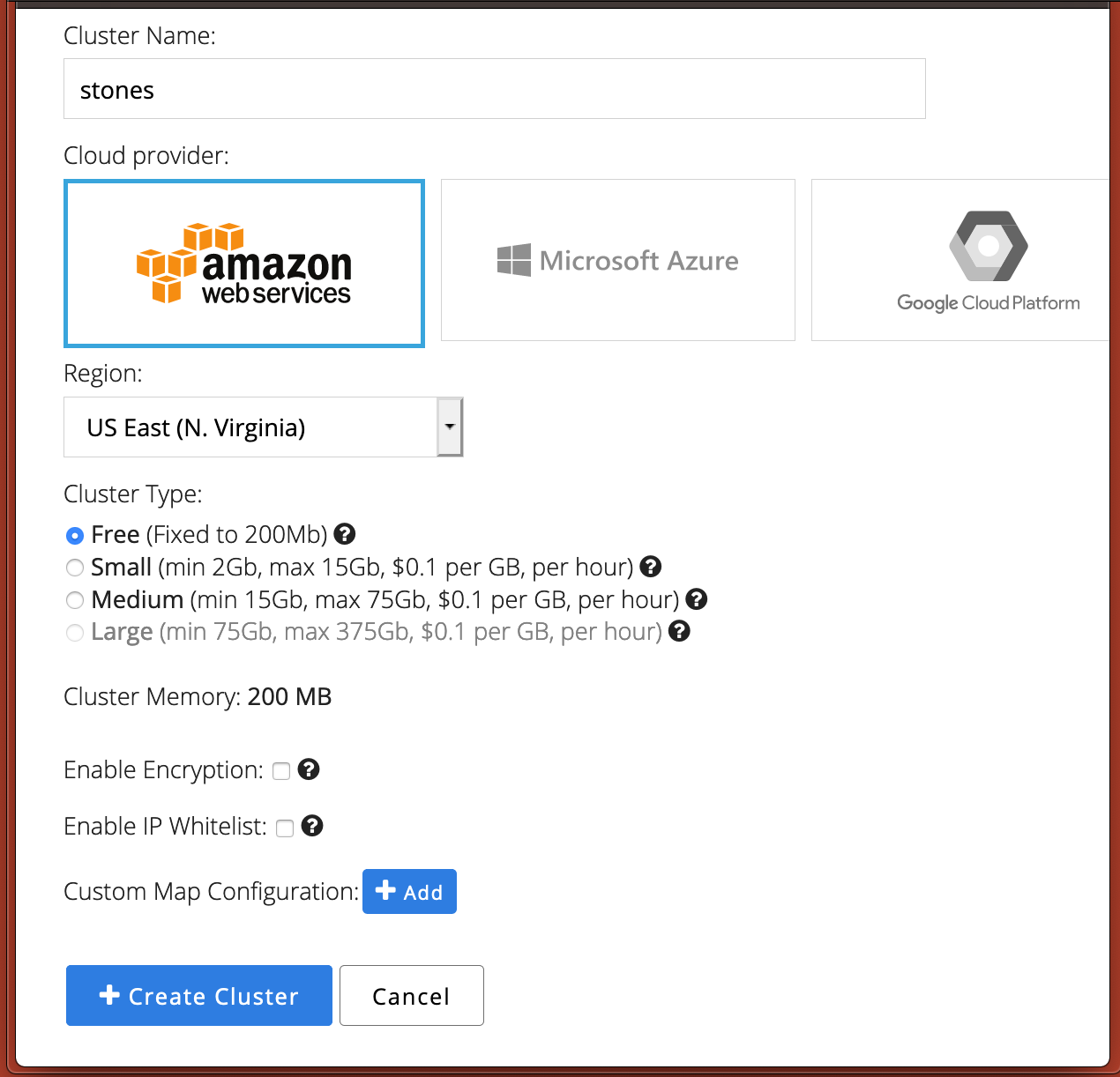
To keep things clear, we’ll create a new cluster without any special customisation. It doesn’t matter what we call it, so we will go with “stones” as a name.
This’ll take a few seconds to create, and once done click on the “Configure Client” button to find out the connection credentials. This will pop up a screen like the below.
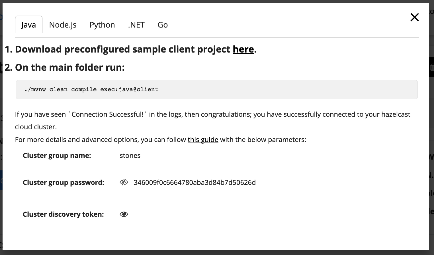
What we need to note is the three fields at the bottom. We need the cluster name ( “stones“), password and discovery token fields. The password and discovery token fields are hidden until you click on the “eye” symbol. Your values will differ of course.
Now we can build and run the client.
mvn install
java -jar target/stdev-0.1-SNAPSHOT.jar
When you start it, you’ll get asked for these three fields:
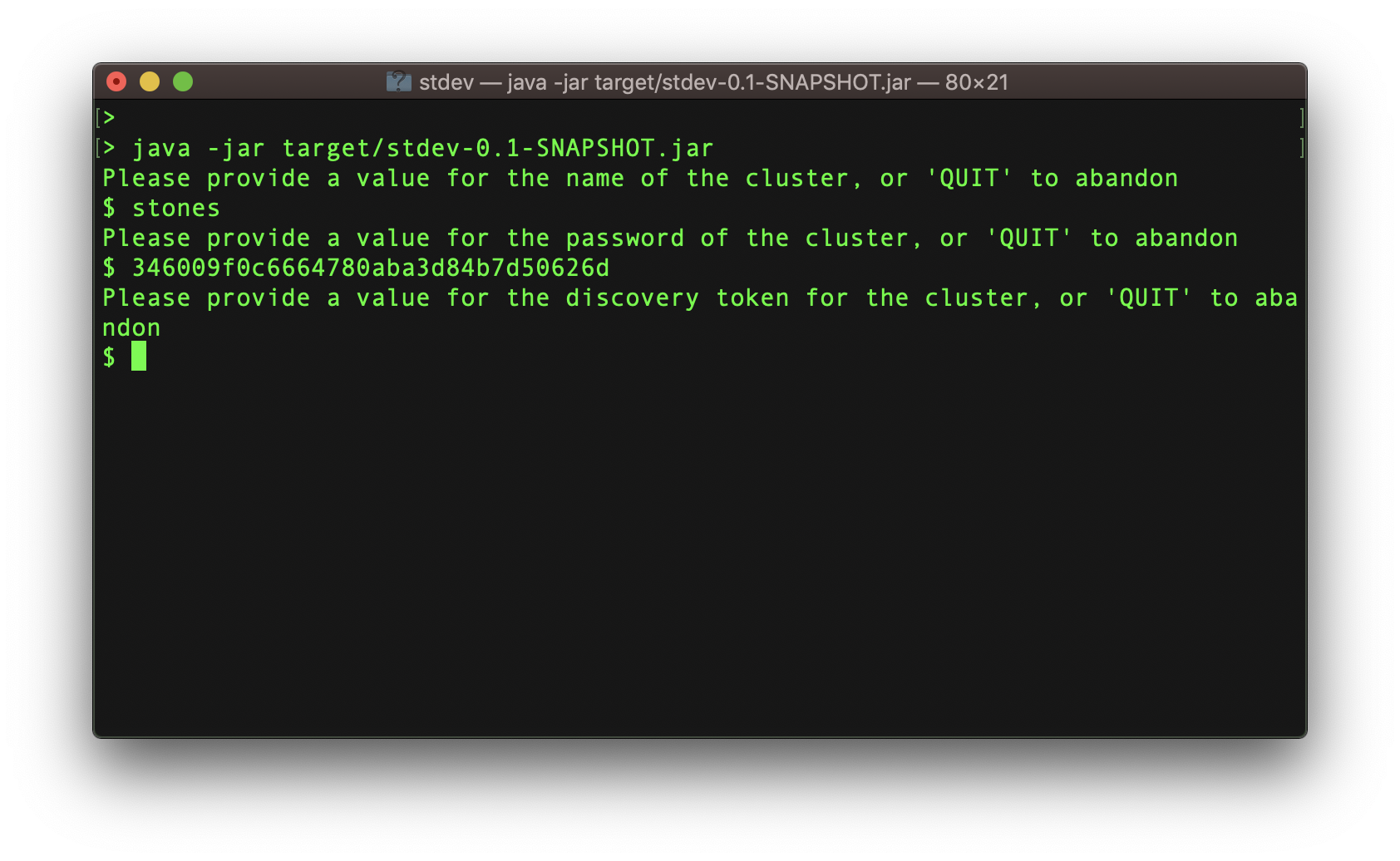
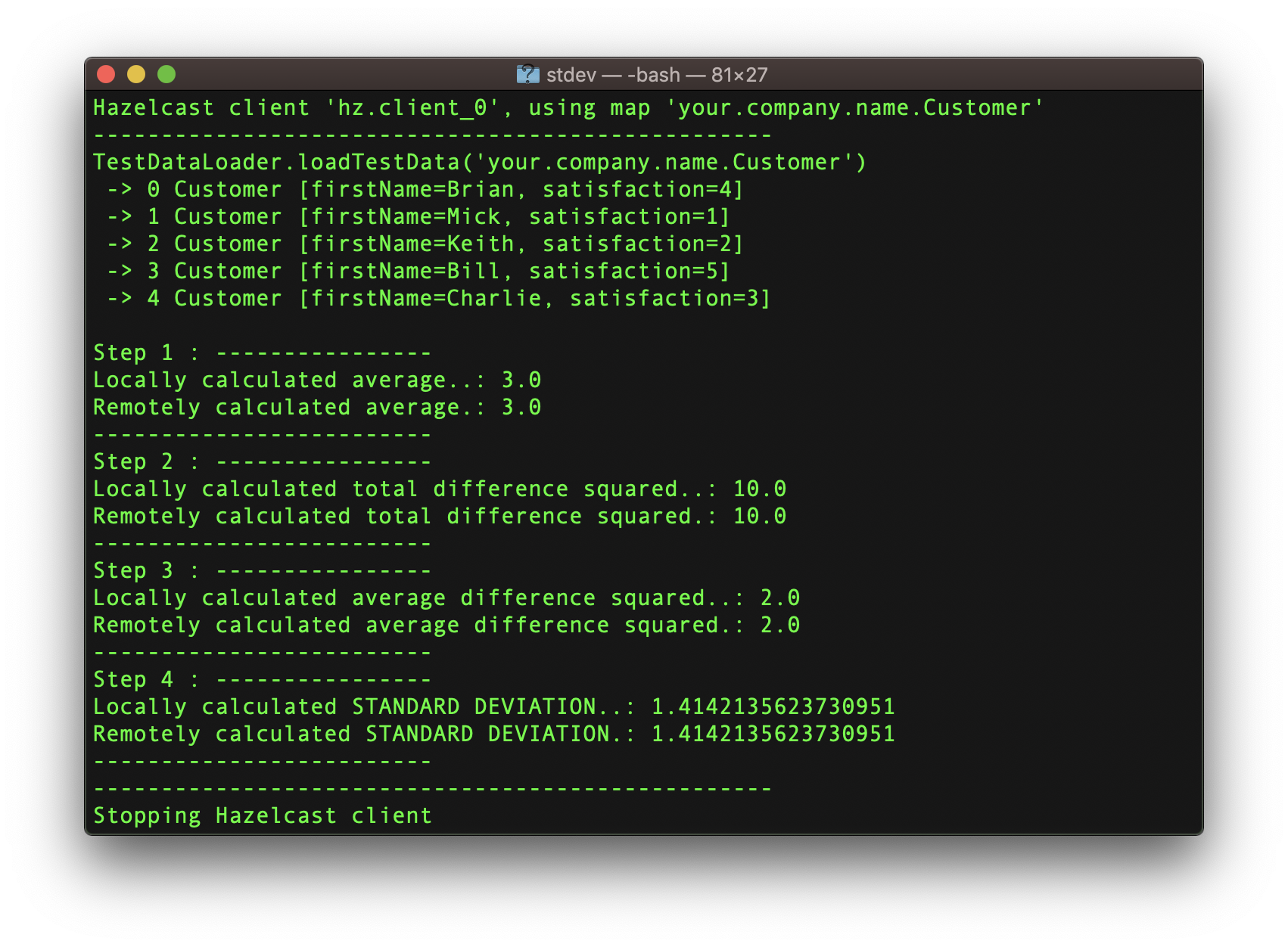
Once these are provided, processing will begin:
Code injection
There is one last point of technical interest. If we are running server-side processing, how do the servers get the code to process?
Typically what we do to “deploy” code is we copy it onto the filesystem on the server machines, and bounce the servers to pick up the code from that filesystem.
This is ok, but it’s not exactly great for high availability.
In Java terms, what this means is we are asking the JVM’s class-loader to read in classes from the filesystem. So we are reading in Java classes from the filesystem, streaming bytes from disk into memory.
Why not stream these bytes from somewhere else?
Streaming bytes is all in a day’s work for Hazelcast!
So what we do here is get our Hazelcast client to send the “Customer.class” and the “TotalDifferenceSquaredCallable.class” to the Hazelcast cluster. This makes these classes available to the class-loader, and therefore to the Hazelcast server. This happens without a restart, which is particularly important if you only have one Hazelcast server process.
If you are interested, the code to do this is in the “ApplicationConfig.java” file, and looks like this:
ClientUserCodeDeploymentConfig clientUserCodeDeploymentConfig = clientConfig.getUserCodeDeploymentConfig();

clientUserCodeDeploymentConfig.setEnabled(true);

clientUserCodeDeploymentConfig.addClass(TotalDifferenceSquaredCallable.class);
clientUserCodeDeploymentConfig.addClass(Customer.class);
We adjust the client’s configuration to say it can send Java classes to the servers, and which particular ones to send.
Summary
This example shows Hazelcast Cloud can be more than a data store or cache. If you want it to be, it can be a compute grid.
This is demonstrated by an example where the business logic is shown the “junior developer” way and the “senior developer” way.
On a cluster with two Hazelcast servers, the senior developer’s way is twice as fast. Expand to three servers and now it’s three times faster than the junior developer’s way. Scalable speed.
One way is better than the other, but which is better depends on whether you value performance or simplicity. The skill of the senior developer is in knowing the choices and using the right one.
Find the sample code here to test data with an average customer satisfaction of 3 with a standard deviation of 1.41. For customer satisfaction, the average is an important metric. But so also is how much variation there is from average, as very unhappy customers consume disproportionate amounts of time.