Bitcoin’s Death Cross

Let’s start off the New Year with a fun code example! This example shows how Jet is used to spot the dramatically-named Death Cross for the price of Bitcoin, which is an indication to sell, Sell, SELL!.

The idea here is that we could automatically analyze stock market prices and use this information to guide our buying and selling decisions.

Disclaimer

This is a code example, not trading advice. Do not use it to make investment decisions. Please!

Background

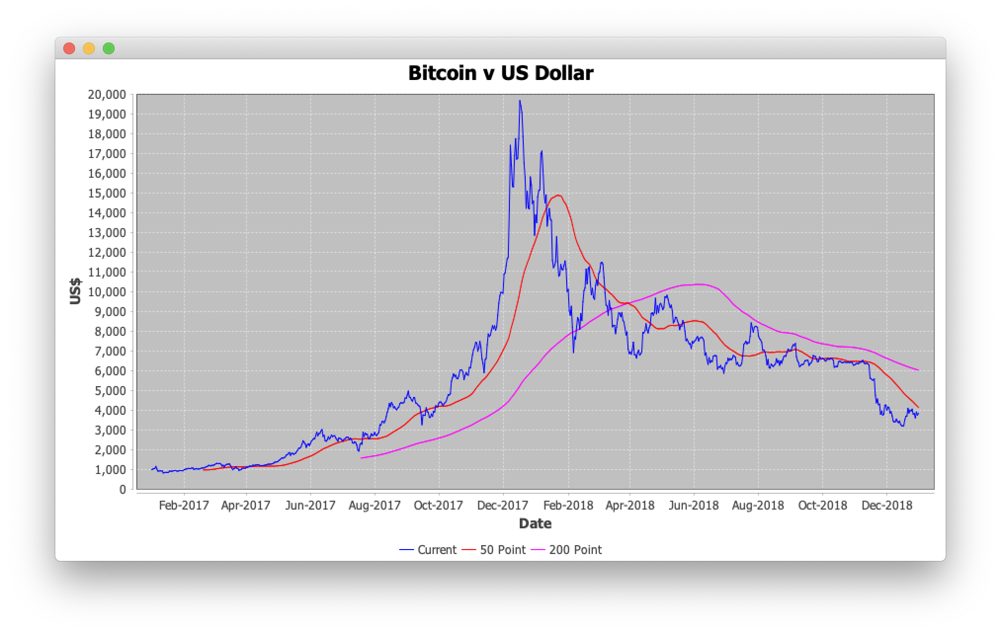
In the graph at the top of this post, the price of Bitcoin is shown as a blue line.

The price goes up and down, and to the human eye, it’s relatively clear that it peaked in December 2017.

So selling in December 2017 might not have been a bad idea, because by January 2018, the price had fallen. But then in February 2018, the price went back up again, so we might have regretted selling.

To confidently buy/sell Bitcoin, we need to study the overall price trend. Is the price going up or down, in general, rather than from moment to moment?

Moving Averages

What we calculate are moving averages to smooth out the variation in the price.

The red line is the “50-Point Moving Average.”

The idea for the 50-point moving average is to take 50 input points and calculate the average, then move 1 point forward and repeat.

We have daily prices, so the first 50 points to average are January 1st, 2017 to February 19th, 2017. The average of these 50 prices is $951.

The next 50 points to average are January 2nd, 2017 to February 20th, 2017. We have moved forward by one input. 49 of the 50 points considered are the same as the previous calculation, so the average will not vary much. This smoothes out variation in the input, giving the output on February 20th, 2017 of $952.

The price of Bitcoin from February 19th-20th, 2017 was a move from $1048 to $1077. The 50 point average has gone from $951 to $952, recognizing an upward trend but a reduction in volatility.

The purple line is the “200-Point Moving Average.” The idea is the same, except it uses 200 points, so it doesn’t begin producing output until July 19th, 2017.

50 and 200 are standard ranges used in investment. The 50-point range gives the short-term trend, while the 200-point range gives the long-term trend.

Death Cross and Golden Cross

What we are looking for is whether the short-term trend and the long-term trend are going in different directions.

On March 30th, 2018, the short-term trend dipped below the long-term trend. This is called the Death Cross.

Later on, in April 2019, they cross the other way, known as the Golden Cross.

Golden Cross and Death Cross indicate positive and negative perspectives on the price. For a trader, both situations means there is money to be made, so both are good news.

What Does Jet Add?

Speed!

The business logic here is just averages; nothing remarkable. The value comes from speed.

We need to detect it in time to sell when others still think buying is a good idea. After all, we can only sell to someone that wants to buy.

If we do this on the price stream as it comes in, we’re going to be faster than those that store the prices to analyze later. Time is money.

Running the Example

From the top-level of the bitcoin-death-cross folder, use:

mvn spring-boot:run

Or, if you prefer:

mvn install
java -jar target/bitcoin-death-cross.jar

What you should see is a graph appear and the prices plotting dynamically.

The prices themselves are stored in the src/main/resources/BTCUSD.csv file, but you could easily convert to connect to a live stock exchange if you wanted.

Understanding the Example

Business Logic

The business logic here is based around trend analysis using the “simple moving average.”

For one 50-point calculation, 50 consecutive prices are added together, and the sum is divided by 50 to give the result. A calculation is made from points 1 to 50, then from 2 to 51, then from 3 to 52, and so on.

But there are plenty of ways we could make the calculation more sophisticated, in the hope of providing better results.

For example, using points 1 to 50 to produce a value, then points 2 to 51 to deliver the next value provides minimal variance. Both calculations use points 2 to 50; only points 1 and 51 differ,  so the output does not vary by much. We might decide to alter the stepping factor from 1 to 2 so there is less overlap when using points 1 to 50, then points 3 to 52, then 5 to 54, then 7 to 56, and so on.

We could also introduce a weighting to reflect the fact that newer prices are more important. We might count the last point twice, for example. Here we would add points 1 to 50 together as before, add point 50 again, and now divide by 51 to get our result. This would no longer genuinely be considered an average.

Map Journal

Hazelcast provides an Event Journal on map and cache data structures.

Our price feed is preset, as it’s just an example. The class com.hazelcast.jet.demos.bitcoin.Task4PriceFeed reads from the CSV file of prices and writes them into a map.

So what the map stores is the current price of Bitcoin. If we do “map.get("BTCUSD")” we get back a single value—the last value written, as you would expect.

But the hazelcast.yaml configuration file tells Hazelcast to track the history of changes to this map, and Jet can process this event log. So now we have access to every value written for each key, depending on the capacity we configure for the event log.

The Jet code to do this is below:

pipeline.drawFrom(
  Sources.mapJournal(
    MyConstants.IMAP_NAME_PRICES_IN,
    JournalInitialPosition.START_FROM_OLDEST)
)

We tell Jet to use the change history for the given map as an infinite input stream. Jet has access to events from before the Jet job started executing (START_FROM_OLDEST) and every update that occurred while the Jet job ran.

Sources.mapJournal() gives a continuous stream of updates to a map, unlike Source.map(), which provides a one-off batch of current map content.

If you want to connect to a live stock exchange, the above is the element that needs to change.

The Pipeline

The data pipeline for this demo is relatively large:

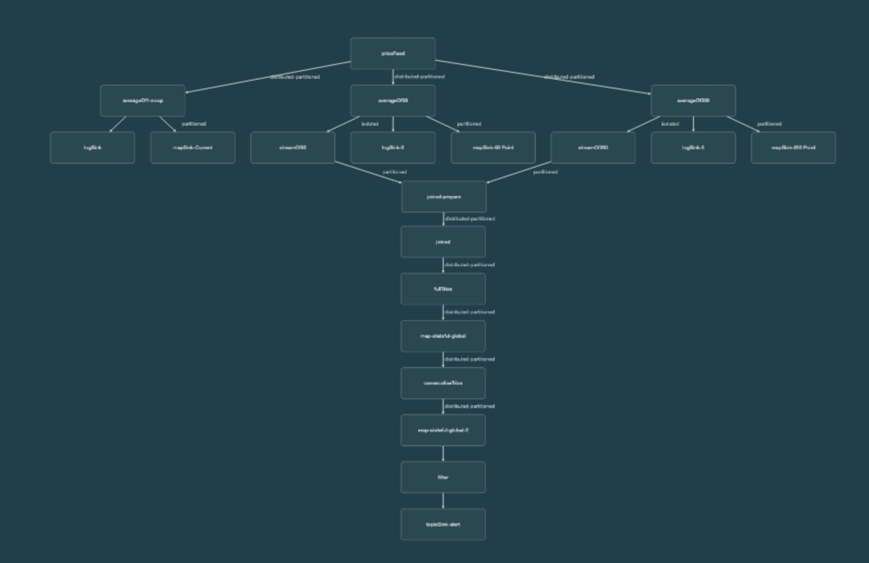
However, that’s because it’s doing various things to make the demo more interesting, like saving the prices to a map so other code can plot the prices on a chart.

There are only four parts of specific interest:

Price Feed

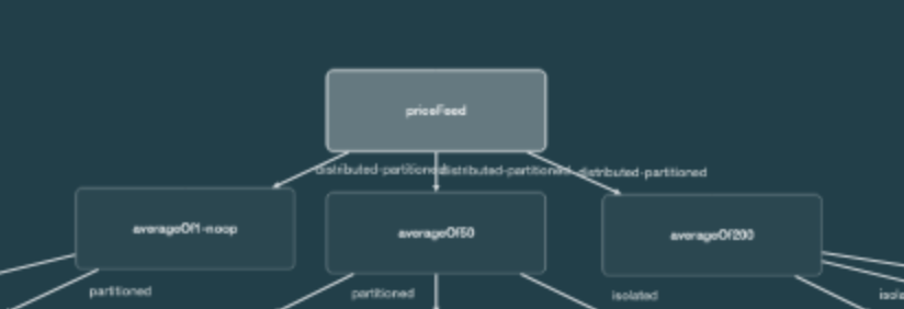
The first stage of the pipeline is, of course, the source. In this case, it’s an infinite stream of prices coming from a map event journal.

A recurring theme for stream processing is reduction. A feed of big data is transformed into meaningful small data by a series of filters, projections, and aggregations.

Here we do the reverse—we increase the data volume. Our single feed of prices broadcasts to three subsequent pipeline steps. For every one price that comes in, three copies of it are sent to later stages in the pipeline.

We do this to calculate the 50-point moving average and 200-point moving average from the same input data. As a bonus, we also calculate the 1-point moving average. The 1-point moving average is, of course, a no-op; each input price produces the same output price, which in this example is a helpful convenience to reformat the input into the output format.

So the code here is:

StreamStage<Entry> averageOf1 =
    MovingAverage.buildAverageOfCount(1, priceFeed);
StreamStage<Entry> averageOf50 =
    MovingAverage.buildAverageOfCount(50, priceFeed);
StreamStage<Entry> averageOf200 =
    MovingAverage.buildAverageOfCount(200, priceFeed);

Moving Average

To calculate the moving average itself, we provide a method to transform the input into the output.

priceFeed.customTransform(
    stageName, () -> new SimpleMovingAverage(count)

This code uses a ring buffer to store the input prices. This is sized at 1, 50, or 200, depending on which average we are calculating.

For each item of input, we add it to the ring buffer, and if it is not full, we indicate to Jet (by returning true) that we have successfully processed the input.

if (this.rates[next]==null) {
    this.current = next;
    return true;
}

Once the ring buffer is full, we can create the average and try to produce the output. This can fail if the output queue for this step is full, so we use this to determine if we successfully processed the input.

Entry result
    = new SimpleImmutableEntry(this.key, average);
                        
boolean emit = super.tryEmit(result);
if (emit) {
    this.current = next;
}
return emit;

Join

From a technical standpoint, the most interesting stage is the join.

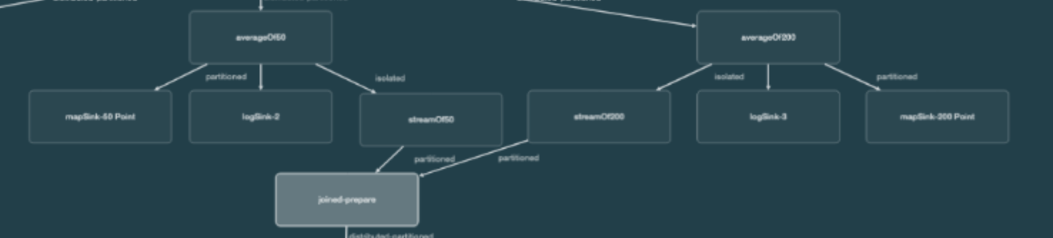
The 50-point moving average stream is producing pairs of dates and prices. The 200-point moving average stream is also producing pairs of dates and prices.

What we want to do is join these on the date, to produce a trio—the date, the 50-point price, and the 200-point price. So our input to the join is two streams.

StageWithKeyAndWindow<Entry, String> timestampedWindowedOf50;
StreamStageWithKey<Entry, String> timestampedOf200;

The left side is the 50-point stream, which is timestamped from the date of the average, the 50th day for the 50-point. It advances in windows of one day, so we get one price at a time since we have daily prices.

The right side is the 200-point stream, which also is timestamped from the date of its average, the date of the last (200th) price.

We join them easily,

windowOf50.aggregate2(windowOf200, myAggregateOperation)

using a 2-stream aggregator. The left side windowOf50 is blended with the right side windowOf200 using a customer aggregation.

The aggregation has three main parts:

public MyPriceAccumulator setLeft(Price arg0) {
    this.left = arg0.getRate();
    this.date = arg0.getLocalDate();
    return this;
}

public MyPriceAccumulator setRight(Price arg0) {
    this.right = arg0.getRate();
    return this;
}

public Tuple3 result() {
    return Tuple3.tuple3(this.date, this.left, this.right);
}

When a left side item arrives, setLeft() is called, and this saves the date and the price from that item (50-point) to instance variables in the aggregator object.

When a right-side item arrives, setRight() is called, saving the price from the 200-point item. We could save the date here too, but it’s the same date as came in on the left side.

Finally, once left and right items have been received, result() is called to make the output. Tuple3 is a utility class provided by Jet for holding trios. There is also Tuple4, Tuple5, etc.

Alerting

The last stage is alerting; there’s no use detecting a Death Cross or Golden Cross if we can’t tell anyone about it.

We create our own sink, to publish to a Hazelcast topic. Any processes with topic listeners, such as Hazelcast clients, would be notified if the Jet job wrote anything to the topic.

SinkBuilder.sinkBuilder(
    "topicSink-" + MyConstants.ITOPIC_NAME_ALERT, 
    context -> 
        context.jetInstance().getHazelcastInstance().getTopic(MyConstants.ITOPIC_NAME_ALERT)
    )
    .receiveFn((iTopic, item) -> iTopic.publish(item))
    .build();

We use the execution context to retrieve a reference to the Hazelcast topic, and if this stage receives an item, it uses the object returned from the context as the place to publish the item.

Does This Work?

Alerts are produced for a downward cross on March 30th, 2018, an upward cross on April 24th, 2019, and another downward cross on October 26th, 2019.

So if you had one Bitcoin to begin with, and sold it for $6853 on March 30th, 2018, you would have $6,853.

$6,853 would have bought 1.26 Bitcoins on April 24th, 2019.

Selling 1.26 Bitcoins on October 26th, 2019 would turn this in $11,629.

If you’d held on to the 1 Bitcoin throughout the time period, by the end of 2019, this would be worth $7,196.

Bitcoin started 2017 at $995, so $7,196 is not bad, but $11,629 is better.

Summary

This example shows how you can derive insights on a stream of data as it arrives, which is vital for time-critical applications. The code is here.

As a reminder, the business logic in the example is pretty flimsy. Do not use it to make investment decisions.

Price trend analysis is a real industry segment, and it just uses better rules.

In the future, we’ll look at $995 US Dollars for 1 Bitcoin with as much amusement as 2005’s $100 US Dollars for 1GB of RAM.