Projections, Joins and Partition Awareness

This example shows some of the newer features of querying, a way that joins can be achieved, and shows the pros and cons of partition aware routing.

Although mainly an Hazelcast IMDG example, Hazelcast Jet puts in a guest appearance to implement the join.

Background – Partitioning

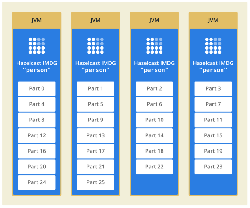
The most commonly used data structure in Hazelcast is com.hazelcast.core.IMap.

An IMap can mostly be used interchangeably as an java.util.Map, as a _key-value_store.

Behind the scenes there are differences. The most important one for this example is that the IMap is partitioned. What we mean by this is the IMap is divided into sections called partitions, and these partitions are spread across the available server JVMs.

In this diagram, there is an IMap called “person” for storing details about people, divided into 26 parts, and spread across 4 JVMs.

 

Scaling

This partitioning gives the benefit of scaling.

No one JVM holds all the IMap content, so more data can be injected into the “person” map than any one JVM can cope with — a significant advantage over java.util.Map.

Furthermore, if servers are added to the cluster, Hazelcast will automatically re-arrange the partitions across the existing and added servers to rebalance the load. So, capacity can be increased or reduced while the cluster runs.

 

Networking

Spreading the data in such a way isn’t problematic for CRUD operations. Typically the caller maintains a connection to every server, so if a data record is needed from the 1st server it’s a single hop across the network. And if the next data record needed from the 2nd server then there’s a connection open to that too and again it’s a single network hop to get it.

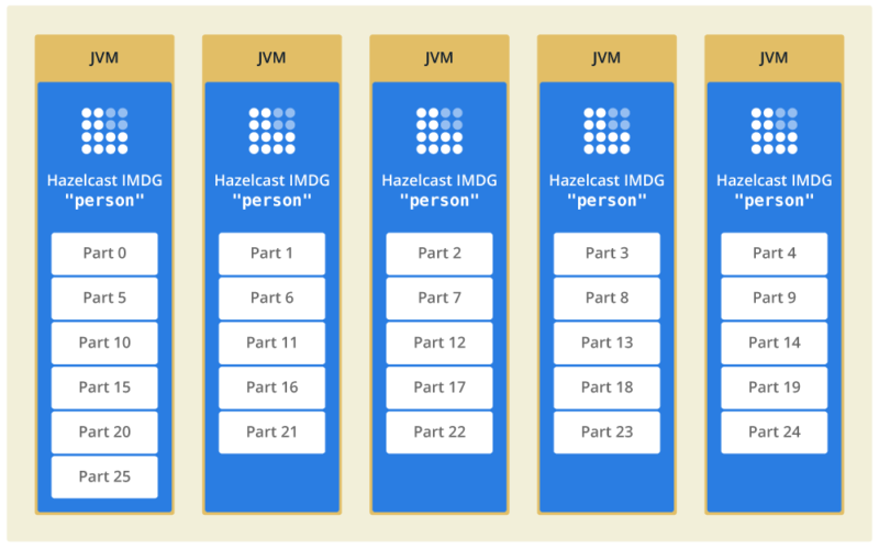
Spreading the data makes querying faster. If we need to search through the data records and there are 5 JVMs (as in diagram 2), the search can run in parallel across all 5 servers at once and complete in 1/5th of the time.

Often processing needs access to several data records at once, and this is hampered if the data records are on different JVMs. Although the network transfer may be fast, it still contributes to run time. Using PartitionAware can help.

Partition Aware

The default algorithm for determining which partition stores a particular data record is based on the whole key of the data record. Simplistically, the entry with key “1” might go to partition 1, key “2” to partition 2, key “3” to partition 3.

What this means in practice is that processing that runs on a server JVM and needs access to entries “1” and “3” will get inconsistent performance. If the partitions containing those entries are hosted by the server JVM on which processing runs, there will be no network transfer of data. If the partitions then get re-arranged to different server JVMs because more server JVMs are added, that same processing will have to retrieve the data across the network, which will give different performance.

The solution here is to use com.hazelcast.core.PartitionAware to override the default algorithm for data placement.

A key that implements PartitionAware has to provide a method getPartitionKey() that provides the routing to Hazelcast. For this example, we might return “odd” for keys “1” and “3“, and “even” for key “2“.

This would ensure that keys “1” and “3” are placed in the same partition. No matter where that partition was hosted, any processing accessing keys “1” and “3” will always find them in the same JVM, and so get consistent performance without networking interference.

This doesn’t affect equality. Keys “1” and “3” are different, separate map entries. They just have the same basis for routing, “odd” instead of the whole key, so have a common destination.

Note also you aren’t specifying which partition they go in, nor where that partition is hosted. It’s just an affinity mechanism.

Partition Aware Detail

The default algorithm for calculating the partition where an entry will reside is to take the hash of the key in binary form, and modulus this by the number of partitions selected.

If that sounds like too much hard work, just ask Hazelcast for the answer:

System.out.println(this.hazelcastInstance.getPartitionService().getPartition("1"));
System.out.println(this.hazelcastInstance.getPartitionService().getPartition("2"));
System.out.println(this.hazelcastInstance.getPartitionService().getPartition("3"));

gives

Partition [41]
Partition [257]
Partition [33]

when using the default set-up of 271 partitions.

Partition Aware Dangers

The use of “odd” and “even” is a deliberately bad example to illustrate the potential pitfalls of overriding the partitioning routing with your own scheme.

If all keys result in “odd” or “even“, then only two partitions will ever contain any data. This results in a significant imbalance in the data.

Adding more servers to increase capacity will be ineffectual. Adding more partitions will be ineffectual.

Projections

Normal Hazelcast queries return whole objects — keys, values or both (entries).

As an optimization, projections are available. These allow you to select the fields you want from the objects being queried for the result set.

If the result set is smaller because it doesn’t contain unwanted fields, then it is quicker to transmit.

Querying on Keys

The IMap is a key-value store. Queries are normally expressed as predicates to match against the value.

Alternatively, the predicate can be coded to match against the key as well.

For equality checking, it would be coded as “__key = 1“. This is pointless, if you have the full key then “IMap.get(key)” will always be faster as it doesn’t have to search.

Where key search is useful is comparison searches (“__key > 1“) and wildcard searches (“__key LIKE "John%"“).

Joins

Joins are more problematic.

Remembering that the main use case for IMap is for scaling, where the data is too voluminous to fit in one JVM, and is split into parts to spread the load of hosting.

It is almost axiomatic that if the data has been split up because it is big, it cannot be joined because it is big.

This is true in general, and so joins are not supported by Hazelcast IMDG. But it is possible in certain specific cases, as we’ll see in the example using Hazelcast Jet.

The example

The example itself uses two main IMaps and derives a third.

The first IMap is called “person” and contains information about people. The key is a compound of first name and last name. The value is the person’s date of birth.

The second IMap is called “deaths” and records the date of death for some of the people. The date of death is held in a separate record from the date of birth; partly to make the example more challenging, and also because not everyone will have died. So this is a de-normalized data model.

The third IMap is called “life“. It holds the age of people at their death, and is derived from the previous two maps, much like a materialized view in a relational database.

Key components

Two parts of the example are worth a closer look:

PersonKey.java

The PersonKey class defines the key for the “person” map. It is compound of first name and last name.

This is defined as PartitionAware and so defines a routing function getPartitionKey() which returns the first letter of the last name.

So for the two people “John Doe” and “Jane Doe“, the partition choice will be based on “D” and both will go to the same partition.

This is (deliberately) a BAD algorithm to chose.

For a start, there are only 26 letters in the western alphabet that will be used for last names. So with the default 271 partitions, 26 could be used and 245 will always be empty.

And furthermore, not all names occur with the same frequency. So the partition holding the people whose last name begins with “M” will likely have a different count than the partition holding those whose last name begins with “P”.

Returning

this.lastName;

instead of

this.lastName.charAt(0);

would be a considerably improvement for balancing the data.

LifeAgeValueExtractor.java

For the “life” map, the data entry is LifeValue which holds the date of birth and the date of death.

What LifeAgeValueExtractor does is make a virtual third field (“age“) at runtime, by subtracting birth from death.

This new field “age” is then usable in queries just like any other.

Running the example

The example uses Spring Boot, so you need to run mvn install to create an executable Jar file.

Then run this command to start a Hazelcast instance:

java -jar target/project-key-0.1-SNAPSHOT.jar 

Ideally run this twice or more at once. The later steps of the example show data distribution across members, so one won’t be enough.

Step 1 – Load Test Data

From any of the running instances, enter “load” as a command on the command line.

Code in TestDataLoader.load() will load 6 records into the “person” map and 4 into the “deaths” map.

Run the “list” command to display this data.

Step 2 – Key Query #1

Run the command “howard” to query for all people who have the last name “Howard”.

The code is in MyCommands.howard() and the important line is this:

new SqlPredicate("__key.lastName = 'Howard'")

This returns all the values in the “person” map that match the above predicate.

As the values only contain the date of birth, this isn’t wonderfully helpful. The output shows the date of birth but not the name.

Step 3 – Key Query #2

Now run the command “howard2“.

This is a refinement to the previous, adding this projection

Projections.multiAttribute("dateOfBirth", "__key.firstName");

So, the query is looking for matches based on last name but returns the first name and the data of birth.

This is more efficient for network transfer than returning the full entry. Less data transfers across the network than returning the entry to the caller only to have some fields not displayed (ie. last name is not printed).

Step 4 – Data Location

Run the location command. For each record in the “person” map, the partition and hosting JVM is printed.

Assuming you are running two or more JVMs at this point you should see some records are on different JVMs.

Because of the PartitionAware coding, you should see all the records for last name “Howard” are in the same partition.

If you can, add or remove some server JVMs for the cluster and rerun this command after the automatic rebalance. Partitions may have moved, and if “Howard” records have moved they are still all kept together.

Step 5 – Join

The “join” command runs a Jet pipeline to pull data from two IMaps and output the result to a third IMap.

In Hazelcast IMDG, joins are not supported. Queries run on a single map at a time, and if data is so big it needs to be distributed onto multiple nodes then in general it is so big that combining two or more maps won’t fit in memory.

This is where Jet lends a hand.

An 8-step Jet pipeline is defined.

• Steps 1 and 2 read from the IMap named “person” and reduce it down to just the fields needed, “firstName” and “dateOfBirth“.
• Steps 3 and 4 do the same for the IMap “deaths” resulting in pairs of “firstName” and “dateOfDeath“.
• Step 5 has two input streams
  • (“firstName“, “dateOfBirth“)
  • (“firstName“, “dateOfDeath“)
  • so the join is easy, and produces ((“firstName“, “dateOfBirth“), “dateOfDeath“)
• Step 6 filters out results where the “dateOfDeath” is null. Step 5 tries to enrich step 2 stream with step 4 stream but there may not always be a match.
• Step 7 and 8 convert the output from step 6 into a map entry and store it in the IMap named “life“.

NB There are 6 rows of test data in the “person” map, and 4 in “deaths“.

So this gives the potential for 24 combinations which isn’t going to overflow memory. Actually there are only 4 matches, so it’s even less.

However, the number of matches fits in memory by luck not design. If more rows of test data are added, at some point the number of results could be too great.

This join happens to work, but it is not guaranteed that it won’t result in an OutOfMemoryError in the future if more data is added.

Step 6 – List

As the join is coded to send output to an IMap the result isn’t immediately visible.

Run the command “list” to output the content of the three maps.

Now that the join has run, the “life” map has been populated.

Step 7 – Oldest

The last step is to find out which of the four entries in the “life” map lived for the longest.

Run the command “longevity”

The code first does

int max = lifeMap.aggregate(Aggregators.integerMax("age"));

to find the oldest age. Remember the “age” field is virtual, it’s not actually a field in the LifeValue object but is derived.

Then

Set<String> keySet = lifeMap.keySet(new SqlPredicate("age = " + max));

is run to find all the people that lived for that long.

Summary

Use of the “__key” prefix allows you to use a key or part of a key in search predicate.

Use of PartitionAware on a key overrides Hazelcast’s data placement rules. This can result in great performance boost by utilising domain specific knowledge, or can go badly wrong.

Projections reduce the size of the result set to the parts you need.

Aggregations do server-side calculations, further reducing the result set that gets sent to the caller.

Joins are not supported, but can be built for specific situations using Hazelcast Jet.